filmov
tv
Excel Magic Trick 1383: Conditional Format Row w OR Logical Test with Multiple Partial Text Criteria

Показать описание
Download Files:
Start File and Finished File:
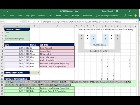
See how to Conditionally Format each row in a Data Set that has a Job Title that contains any text item from within a list. Learn about “Contains Criteria” in an OR Logical Test:
1. (00:11) Introduction
2. (02:53) OR, ISNUMBER and SEARCH functions in an Logical Array Formula that requires Ctrl + Shift + Enter (in the cells). Learn how Array Formulas that require Ctrl + Shift + Enter will work in the Conditional Formatting Dialog Box.
3. (08:45) Convert Contains Criteria list to an Excel Table to allow the list of criteria to expand or contract.
4. (10:13) LOOKUP and SEARCH functions in an Logical Array Formula that does NOT requires Ctrl + Shift + Enter (in the cells). Learn how the Big Number 2^15 can be used in an Approximate Match Lookup Formula when searching for text in a cell.
5. (13:35) Summary
6. Not in video, but in the downloadable Workbook compare and time the LOOKUP Formula using either SEARCH or MATCH functions.
Alternative Title: Excel Magic Trick 1383: Conditional Format Row w OR Logical Test Multiple Contains (Partial Text) Criteria
Match Job Title to List of Key Words
Start File and Finished File:
See how to Conditionally Format each row in a Data Set that has a Job Title that contains any text item from within a list. Learn about “Contains Criteria” in an OR Logical Test:
1. (00:11) Introduction
2. (02:53) OR, ISNUMBER and SEARCH functions in an Logical Array Formula that requires Ctrl + Shift + Enter (in the cells). Learn how Array Formulas that require Ctrl + Shift + Enter will work in the Conditional Formatting Dialog Box.
3. (08:45) Convert Contains Criteria list to an Excel Table to allow the list of criteria to expand or contract.
4. (10:13) LOOKUP and SEARCH functions in an Logical Array Formula that does NOT requires Ctrl + Shift + Enter (in the cells). Learn how the Big Number 2^15 can be used in an Approximate Match Lookup Formula when searching for text in a cell.
5. (13:35) Summary
6. Not in video, but in the downloadable Workbook compare and time the LOOKUP Formula using either SEARCH or MATCH functions.
Alternative Title: Excel Magic Trick 1383: Conditional Format Row w OR Logical Test Multiple Contains (Partial Text) Criteria
Match Job Title to List of Key Words
 0:14:10
Excel Magic Trick 1383: Conditional Format Row w OR Logical Test with Multiple Partial Text Criteria
 0:07:59
Dynamic Excel Multiplication Table with Conditional Formatting. Excel Magic Trick 1683.
 0:38:13
Excel Magic Trick 1382: Extract Records With Multiple Contains (Partial Text) Criteria: 4 Examples
 0:10:51
Excel Magic Trick 1400: Conditionally Format Row in Class Enrollment Table with Complex Criteria
 0:19:34
Excel Magic Trick 1400 Part 2: Conditionally Format Row with Complex Criteria (3 More Examples)
 0:05:21
Excel Magic Trick 1119: Conditional Format Date when 44 Days Have Passed
 0:04:00
Excel Magic Trick 1384: Import Excel Table or Sheet in Power Query or Power BI?
 0:09:49
Excel Magic Trick 1509: Conditional Format Array Formula to Highlight Row With 2 Lookup Values
 0:55:04
Excel Magic Trick 1375 Add w OR Logical Test from 2 Different Columns in 2 Diff. Tables (6 Examples)
 0:17:10
Excel Magic Trick 1359: Split Times Values Into 8 Equal Zones: VLOOKUP, LOOKUP or INT/HOUR?
 0:03:34
Conditional Text in Excel
 0:16:54
Excel Magic Trick 1376: Complex VLOOKUP Formula To Create Transaction Description
 0:20:12
Excel Magic Trick 1482: SUMPRODUCT, DCOUNTA or SUM & IF for Counting with OR Logical Test
 0:03:12
Excel for Schools: Sorting by Conditional Formatting
 0:01:13
2 Comments on Excel Magic Trick 1381
 0:01:21
How to Apply Conditional Formatting to Blank Cells
 0:12:03
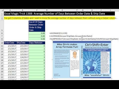
Excel Magic Trick 1388 Average Number of Days Between Order & Ship Date (Basic Array Formula Les...
 0:18:09
Excel Magic Trick 1445: Single Cell Array Formula: Count Customer Names for 8 Sales Coupon Groups
 0:01:44
How to use Conditional Formatting for Between Alphabets in MS Excel 2016
 0:04:41
Excel Magic Trick 1404: Sales Per Working Day by Month using Power Query
 0:02:23
MS EXCEL: CONDITIONAL FORMATTING BETWEEN
 0:04:45
Compare Multiple Excel Cells with Conditional Formatting
 0:51:33
Conditional Formatting in MS Excel- Beginner To Advanced
 0:03:21
Excel Magic Trick 1457 Part 2: Regional Settings & Text or Number Date / Times in SUMIFS Functio...
Комментарии