filmov
tv
Excel Filter By Month: Filter feature or FILTER function? Amazing Dynamic Formula Solution. EMT 1796

Показать описание
Learn how to filter a data set by month using the Filter feature and the FILTER function. See how to create dynamic Data Valication also..
Topics:
1. (00:00) Introduction
2. (00:17) Filter Feature for a data set with just one year of data
3. (01:20) Filter Feature for a data set with multiple years in in data set
4. (02:00) Create Dynamic Data Valication Dropdown List for Year and Month See the functions: SORT, TEXT, UNIQUE
5. (05:16) Create Filtering Formula using the functions: FILTER and TEXT
6. (06:07) Add new records to table and test if solution is dynamic
7. (07:07) Summary,
8. (07:26) Closing, Video Links
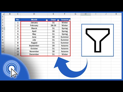
Filter Your Data by Month in Excel
Excel Filter By Month: Filter feature or FILTER function? Amazing Dynamic Formula Solution. EMT 1796
Excel Pro Tricks: Dynamically Filter Data based on Month with FILTER function in Excel Formula
Dynamically Filter Data based on Month with FILTER function in Excel
Excel Date Filter Magic - Last Month, This Month, YTD & More + Awesome Interface
DATE GROUP IN EXCEL | group date in autofilter menu excel | ADVANCE setting |filter excel
Apply Smartly Date Filter in Excel
MS Excel - Filtering Data
Data Cleaning/Extraction with Regex in Excel | Sumit Bansal
How to Create Filter in Excel
Excel FILTER Function
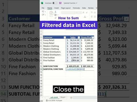
How to sum filtered data in Excel
Filter Function Date Range Criteria in Excel
How To Use Excel FILTER Function With Multiple Criteria & Return Only the Columns You Need
Excel Slicers containing Year and Month
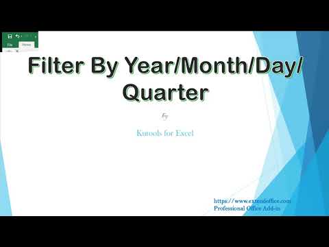
Quickly filter data by year/month/day/week/quarter in Excel
How to sort by date in Microsoft excel
Excel Pivot Tables: How to Group Dates into Years and Months
Excel Filter Function: Filtering Top Grade Students
Quick way to filter data in #excel #spreadsheet #excelhelp #corporatehacks
Filter Pivot Tables For Month-to-date Mtd Comparisons With Slicers
Excel: Year/Month/Day- Custom AutoFilter for date columns
Elegant Date and Location Filtering in Excel - A Must See!
How to Create a Roll up by Month Filter in an Excel Pivot Table
Комментарии
 0:05:14
 0:07:50
 0:00:50
 0:00:44
 0:26:47
 0:03:04
 0:00:44
 0:07:10
 1:04:10
 0:02:51
 0:00:33
 0:00:32
 0:03:15
 0:09:52
 0:05:59
 0:01:14
 0:01:26
 0:01:02
 0:00:28
 0:00:18
 0:09:28
 0:03:25
 0:14:39
 0:05:43