RBC Baseline Model in Dynare: Deterministic vs Stochastic Simulations

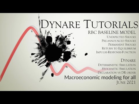
This video is part of a series of videos on the baseline Real Business Cycle model and its implementation in Dynare. In this video I focus on simulations and discuss the difference between the deterministic and stochastic model framework of Dynare. I provide intuition how Dynare "solves" or "simulates" these different model frameworks and guidance on when to run either deterministic or stochastic simulations. Then I show how to simulate various scenarios in the baseline RBC model.

In the **deterministic** case (i.e. under perfect foresight), this videos covers
- unexpected or pre-announced temporary shocks
- unexpected or pre-announced permanent shocks
- return to equilibrium
by using Dynare's `perfect_foresight_setup` and `perfect_foresight_solver` (i.e. the old `simul`) commands and the `shocks`, `initval`, `endval` and `histval` blocks. I show what happens in MATLAB's workspace and to Dynare's output structure `oo_`.

In the **stochastic** case, this videos covers
- impulse-response-functions (irf)
- variance decompositions
- theoretical vs. simulated moments
- data simulation
by using Dynare's `stoch_simul` command and the `shocks` block. I show what happens in MATLAB's workspace and to Dynare's output structures `oo_` and `oo_.dr`. Lastly, the difference between Dynare's *declaration* and *DR* (decision-rule) ordering of variables is covered.

**Timestamps**

*Theory*
01:06 - Deterministic vs. stochastic model framework
08:01 - When to use which framework?

*Deterministic Simulation in Dynare*
11:47 - Overview of Dynare commands for deterministic simulations
13:58 - Getting ready in Dynare
15:00 - Scenario 1: Unexpected temporary TFP shock
15:25 - What does `perfect_foresight_setup do?
17:39 - What does `perfect_foresight_solver` do?
19:12 - What happens in MATLAB's workspace?
19:54 - What happens in Dynare's output structure `oo_`?
21:43 - `Simulated_time_series` is a *dseries* object
22:51 - Scenario 2: Sequence of temporary pre-announced shocks
24:56 - Why `simul` is a depreciated syntax; better use `perfect_foresight_setup` and `perfect_foresight_solver`!
26:20 - `dsample` command
27:14 - Scenario 3: Unexpected permanent shock
28:47 - Values of 0 can cause errors as log(0) is inf; double check your `initval` and `endval` blocks!
30:45 - Don't forget to adjust steady-state computations to be dependent on value of exogenous variables (if they are different than 0)
32:27 - Scenario 4: Pre-announced permanent shock
34:07 - Scenario 5: Return to Equilibrium

*Stochastic Simulation in Dynare*
36:26 - Overview of Dynare commands for stochastic simulations
38:28 - Impulse-Response-Function (IRF) of TFP shock
39:39 - Adding a preference shock to the model
41:38 - Impulse-Response-Function (IRF) of preference shock
42:08 - What happens in MATLAB's console?
42:35 - Theoretical moments with `periods=0` option
43:06 - What happens in Dynare's `oo_` structure
43:51 - What happens in Dynare's `oo_.dr` structure
44:53 - Difference between declaration and DR (decision rule) order
46:07 - Simulate data and simulated moments with `periods` option

*Outro & References*
47:01 - Outro
47:52 - References

**Hints & Corrections**
- Don't save you mod files on cloud storage or network drives

[douglasaraujo]

Wow, that’s a great series of videos! Many thanks for explaining this topic so clearly.

[FaisalQuaiyyum]

Thanks Professor. It was very helpful. I encountered one issue: the MATLAB is stating that it does not recognize the dsample function. What to do?

Thanks soo much! You are doing god work making this available !

[Aragorn...]

Well done, Sir. Great explanations!!! Keep up the good work and more videos about DSGE with Dynare, please :)

P/s: the new haircut is way cooler haha

[cz]

Hi professor, thanks for your lectures. I notice that you mentioned that there would be videos covering topics like linearization and log linearization. I wonder if these videos have already come out. I did not find them anywhere.

[ful]

Thank you for all these videos that you have created, they are awesome!! I have a doubt: I don´t understand how to distinguish in Dynare a "unexpected shock" from a "Pre-announced shock". The commands seems the same for me.

[lawrenceogbeifun]

Thank you for the video. A quick question:

I noticed that in your deterministic simulation, the exogenous variable is epsilon_a. My earlier intuition was that in the deterministic model, there are no shocks. i.e., the policy variable is what we use as an exogenous variable. Hence, the shock is simply by changing the values of the exogenous variable. I have seen this approach in some other textbooks and videos on deterministic simulation. Is both approach the same?

[xixi]

Thanks a lot for the video. May I know what the simulated endogenous variable is? e.g. periods = 30. for y, there are 30 values of simulated y

I also find that the irf for the stochastic case and the deterministic case is the same, with all the code the same except the simul and stoch_simul commands..

[xixi]

Thank you very much for the video. I’m a newbie, and very new the idea of simulation. I’m kind of confused that why is the perfect foresight simulation a two point boundary problem. What values can the initial point and end point be, does the end point has to go back to (new) steady state? What if the period is very small, like 3 periods (before the shock went out), will the end point still be needed to go back to the steady state?
Also, in the stochastic situation, is the irf means only give a shock of the size of the standard error only at the first period and can I have irf= 30 and periods =100 both on, ‘cause I saw when you set irf you set periods to be 0 etc. Thanks a lot.

[tsitoha.andriamiharivolamena]

Thanks for your nice and very clear video.
I have a question. I'm trying to use the temporary and permanent chocs in the log-linearized Smets-Wouters model but I'm facing to an issue because Dynare can't found a solution. Is there a specific way to simulate the temporary and permanent chocs in log-linearized DSGE model ? However, there is no issue when I use the Stochastic Simulations to obtain the irf. The obtained irf with the stochastic simulation is good but I really need the one obtained with deterministic simulation. Idem for the permanent choc. Could you help me please ?
Thanks

[saidul]

Hi Professor, appreciate you for making the great videos!
I have a quick question regarding the shock - how to determine the size of the shock? Do the forms of the model variables (e.g. level vs log) have anything to do with the size of the shock?

[xixi]

may I also consult that, when you set irf=0, periods = 3000, and there are two shocks a and z in the model, may I know what's the simulated value of y, is this y the the simulated value calculated from the policy function from shock a or the shock z? what's the simulated value of y. thanks a lot.

[xixi]

I like the second one, but can I have a third choice :P