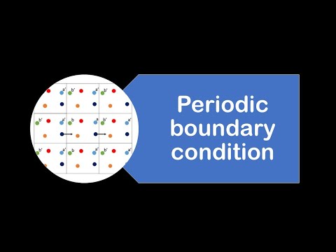
Molecular Dynamics Simulation with Periodic Boundary Conditions

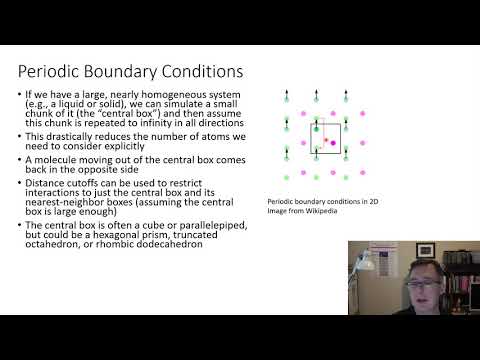
This short clip is intended to illustrate the effects of using periodic boundary conditions for molecular dynamics in 2D. The particles interact as if the simulation box repeats infinitely in all directions. When a particle leaves the simulation box at one end, it appears on the other side.
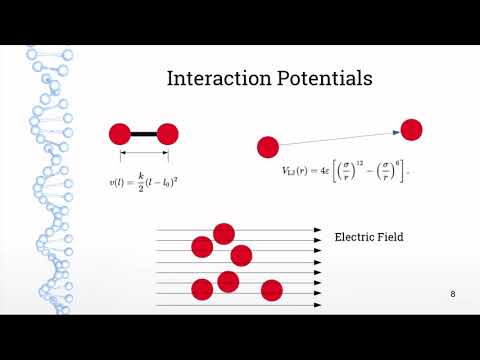
In this case, the particles interact via a Lennard-Jones potential and the Coulomb potential. With periodic boundary conditions, we need to consider the forces across the boundaries, because if the particles simply appeared on the opposite side, a collision could occur, causing the kinetic energy to explode due to the repulsive part of the Lennard-Jones potential scaling with the particle distance to the 12th power!

The implementation is surprisingly simple. First, we have to move the particles that have left the simulation box to the corresponding position on the opposite side. We can use the modulo operator for this, which solves the problem elegantly.
Performing the element-wise modulo operator provides the correct new position inside the simulation box for all particles that have left the boundaries after the integration of the equations of motion in the current time step, while the particles still inside the box remain unaffected.

In Matlab and in 2D:
x_pos = mod(x_pos, box_x_length)
y_pos = mod(y_pos, box_y_length)

That's it for the positions. In contrast to the remainder operation, the modulo operation automatically handles both directions in each dimension.

Now comes the harder part: accounting for the forces across the boundaries. The good news is that once we understand the one-dimensional case, we can simply do the same for all other dimensions and we're done.
The principle is to choose the shortest distance between the particles, as this interaction generates a stronger force and is therefore more important. See minimum image convention. To check whether the inter-box distance is shorter than the distance across the boundaries, we can normalize the inter-box distance to the total size of the box, which gives a value between 0 and 1. If the value is greater than 0.5, the distance across the boundaries must be selected as it is shorter.

The implementation is again surprisingly simple. The round() function can be used to construct a logical vector that only moves the necessary distances. It returns 0 if the distance between the boxes is smaller than 0.5, and -1 or +1 if it is greater. The round() function retains the sign, which automatically reverses the direction of the distance vector when the "clone" particle in the virtual box is closer. (Which is not so important, as it will be squared later anyway, but is still nice)

In Matlab and in 2D:
dx = dx - box_x_lenght*round(dx/box_x_length)
dy = dy - box_y_lenght*round(dy/box_y_length)

After that the Euclidean distance and force can be computed as usuall.

This code was written and executed in Matlab.

[Manabender]

Wouldn't a given particle feel a force from another given particle an infinite number of times? A given particle "sees" infinite copies of another given particle over the boundary, after all.

Is there a simple way of cancelling (nearly) all of these forces out and leaving just a finite number left to calculate?

[tarunsingh]

There was a game called chain reaction …. Same animations