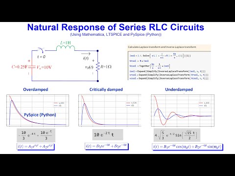
Demystifying Natural Response of Series RLC Circuit Using Mathematica, PySpice (Python) and LTSPICE

This video explains how to make sense of the natural response of a series RLC circuit. It shows how the general solution can be calculated and simulated using Mathematica, PySpice (Python) and LTSPICE. It has the following chapters:
(00:00) [1] Introduction
(01:59) [2] Natural Response Parameters
(06:41) [3] Natural vs. Step Response
(07:42) [4] Laplace Transform
(09:51) [5] Mathematica Demo
(12:04) [6] LTSPICE demo
(12:51) [7] PySpice demo

The Python code and Mathematica code are available in the comments section.

[14/6/2023] Python code modified to also plot the simulated current in the series RLC circuit.

[shubham]

Amazing tutorial! Do we need to be very well-versed with the Python coding to learn PySpice or we just need to know the basics?

[electriccircuits]

Vo = 10;
R = 1;
L = 1;
\[DoubleStruckCapitalC] = 1/4;
StringTemplate[
"Series RLC circuit with R=`1`\[CapitalOmega], L=`2`H and \
C=`3`F"][R, L, \[DoubleStruckCapitalC]]
\[Alpha] = R/(2 L);
StringTemplate["Neper frequency \[Alpha]=`1` rad/s"][\[Alpha]]
\[Omega]0 = 1/Sqrt[L \[DoubleStruckCapitalC] ];
StringTemplate[
"Resonant frequency \!\(\*SubscriptBox[\(\[Omega]\), \(o\)]\)=`1` \
rad/s"][\[Omega]0]
\[Zeta] = \[Alpha]/\[Omega]0 // N;
StringTemplate["Damping factor \[Zeta]=`1`"][\[Zeta]]
Which[\[Zeta] == 1, Text[Critically damped], \[Zeta] < 1,
Text[Underdamped], \[Zeta] > 1, Text[Overdamped]]
If[\[Zeta] < 1, \[Omega]d = Sqrt[\[Omega]0^2 - \[Alpha]^2];]
If [\[Zeta] < 1,
StringTemplate[
"Damped frequency \!\(\*SubscriptBox[\(\[Omega]\), \(d\)]\)=`1` \
rad/s"][\[Omega]d]]
s1 = -\[Alpha] + Sqrt[\[Alpha]^2 - \[Omega]0^2];
s2 = -\[Alpha] - Sqrt[\[Alpha]^2 - \[Omega]0^2];
StringTemplate[
"The roots of chracteristic equation are \!\(\*SubscriptBox[\(s\), \
\(1\)]\)=`1` and \!\(\*SubscriptBox[\(s\), \(2\)]\)=`2`"][s1, s2]
\[CapitalIota]sol = \[CapitalIota] /.
Solve[ s L \[CapitalIota] + \[CapitalIota]/(
s \[DoubleStruckCapitalC]) + R \[CapitalIota] == Vo/
s, {\[CapitalIota]}][[1]]
Vrsol = R*\[CapitalIota]sol
Vcsol = Together[
Vo/s - 1/(s
isol = Expand[
Simplify[InverseLaplaceTransform[\[CapitalIota]sol, s, t]]]
vrsol = Vrsol, s, t]]]
vcsol = Vcsol, s, t]]]
p1 = Plot[{vcsol, vrsol}, {t, 0, 10},
PlotLegends -> {"v_C(t)", "v_R(t)"}, PlotRange -> Full,
AxesLabel -> {"Time (s)", "Voltage"}, AspectRatio -> Full ];
p2 = Plot[{isol}, {t, 0, 10}, PlotLegends -> {"i(t)"},
PlotRange -> Full, AxesLabel -> {"Time (s)", "Current"},
AspectRatio -> Full ];
GraphicsRow[{p1, p2}, ImageSize -> 600]


# Pyspice (Python) code to simulate Natural Response of Series RLC Circuit

# STANDARD DECLARATIONS

import math
import cmath
import matplotlib.pyplot as plt
import numpy as np

import PySpice.Logging.Logging as Logging
logger = Logging.setup_logging()

from PySpice.Probe.Plot import plot
from PySpice.Spice.Library import SpiceLibrary
from PySpice.Spice.Netlist import Circuit
from PySpice.Unit import *
from matplotlib.widgets import Cursor
from engineering_notation import EngNumber
from matplotlib.ticker import EngFormatter


# CIRCUIT NETLIST
circuit = Circuit('Natural Response of Series RLC Circuit')


Vo = 10;
Lvalue=1;
Cvalue=1/4;

# overdamped; any value over 4 Ohm
#Rvalue =5;

# critically damped
#Rvalue=4;

# underdamped; any value less 4 Ohm
Rvalue = 1;
# Rvalue =0;


circuit.PulseVoltageSource(1, 'control', circuit.gnd, initial_value=-1, pulsed_value=1,
pulse_width=finaltime, period=finaltime, delay_time=switchingtime)

circuit.VoltageControlledSwitch(1, 'inp', 'temp', 'control', circuit.gnd, model='switch')

simulator = circuit.simulator(temperature=25, nominal_temperature=25)

analysis = simulator.transient(step_time=steptime, end_time=finaltime)


# THEORETICAL CALCULATIONS

time=np.array(analysis.time)

alpha =
omega0 =
damping_ratio = float(alpha/omega0)

print('Neper frequency, alpha ={}
print('Resonant frequency, omega_0 ={}
print('Damping ratio


if damping_ratio == 1:

print('Series RLC circuit is critically damped')

s1 = -alpha + np.sqrt(alpha**2-omega0**2)
s2 = -alpha - np.sqrt(alpha**2-omega0**2)
print('Root of characteristic equation is s1 ={}'.format(EngNumber(s1)))
print('Root of characteristic equation is s2 ={}'.format(EngNumber(s2)))
D2 = 0
D1 = Vo/Lvalue
print('D1 ={}'.format(EngNumber(D1)))
print('D2 ={}'.format(EngNumber(D2)))
i_out =
v_out = Rvalue* i_out

elif damping_ratio > 1:

print('Series RLC circuit is overdamped')

Vf = Vo
s1 = -alpha + np.sqrt(alpha**2-omega0**2)
s2 = -alpha - np.sqrt(alpha**2-omega0**2)
print('Root of characteristic equation is s1 ={}'.format(EngNumber(s1)))
print('Root of characteristic equation is s2 ={}'.format(EngNumber(s2)))
A2 = (1/(s2-s1))*Vo/Lvalue
A1 = -A2
print('A1 ={}'.format(EngNumber(A1)))
print('A2 ={}'.format(EngNumber(A2)))
i_out = A1*np.exp(s1*time) + A2*np.exp(s2*time)
v_out = Rvalue* i_out

else:

print('Series RLC circuit is underdamped')

omegad=
print('Damped frequency, omega_d ={}
s1 = -alpha +
s2 = -alpha -
print('Root of characteristic equation is s1 ={}'.format(s1))
print('Root of characteristic equation is s2 ={}'.format(s2))
B1 = 0
B2 = Vo/(Lvalue* omegad)
print('B1 ={}'.format(EngNumber(B1)))
print('B2 ={}'.format(EngNumber(B2)))
i_out = B1 * np.exp(-alpha * time) * np.cos(omegad * time) + B2 * np.exp(-alpha * time) * np.sin(omegad * time)
v_out = Rvalue* i_out



# PLOTTING COMMANDS

figure = plt.subplots(3, 1, gridspec_kw={'height_ratios': [1, 3, 1]})

axe1 = plt.subplot(311)
formatter0 = EngFormatter(unit='s')

plt.title('Switch activation')
plt.ylabel('Voltage [V]')
plt.grid()
plot(analysis['control'])
axe1.set_yticks([-1, 0, 1])

axe2 = plt.subplot(312)
formatter1 = EngFormatter(unit='s')

plt.title('Voltages')
plt.xlabel('Time')
plt.ylabel('Voltage [V]')
plt.grid()
plot(analysis['inp'], color='red')
plot(analysis['output'], color='black')
plt.plot(time, v_out, 'b:')
plt.legend(('v_C(t) - simulation', 'v_R(t) - simulation', 'v_R(t) - theory'), loc=(.6, .6))
cursor = Cursor(axe2, useblit=True, color='blue', linewidth=1)

## Plot the simulated current in the series RLC circuit
axe = plt.subplot(313)
plt.xlabel('Time')
plt.ylabel('Current [A]')
plt.grid
formatter0 = EngFormatter(unit='s')

i=
plt.plot(time, i, 'b-')
plt.show()