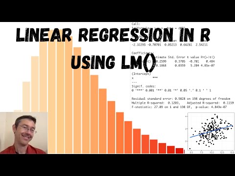
R Tutorial : Basic lm() functions with glm()

---

Welcome back. During the previous exercises, you learned about Poisson regressions. Now, you will learn how lm() functions can be applied to glm()s. These functions help to understand and use GLM outputs.

Base R has many functions for interacting with linear models, and by extensions GLMs. In fact, both LMs and GLMs form a backbone of R and its predecessor S. The original authors of these languages often used LMs. These functions allow us to easily access some parts of models. Thus, rather than needing to manually interrogate and extract model outputs, R gives helpful shortcuts. These shortcuts allows us to see the model outputs with function like print() and also make statistical inferences with function like summary().

When we run a GLM, model output automatically appears, just like a LM.

Alternatively, we can explicitly print model output using the print function.

This output tells us several useful things including what model was fit or "call"ed; the estimated coefficients; the degrees of freedom (which can be thought of as how many "extra" observations we have); the null deviance and residual deviance (which is the GLM version of residuals); and the AIC score for the model.

In contrast to print(), summary() provides more details.

The first part of a summary output is the same as print and I did not include it to save space.

The next portion of the glm() summary() includes a summary of the deviance residuals, which can be helpful for understanding a model fit.

Next, summary displays coefficients as well as their standard errors, z-scores, and p-values.

These can tell us if coefficient explains more variability than would be expected by chance alone.

Next, summary() tells us about dispersion.

Although not covered in this course, some data can be over-dispersed and either have more variance or zeros than the model suggests.

These models require special over-dispersion parameters.

Next, the model provides us similar deviance and degrees-of-freedom information as the print() output.
Last, summary() provides us with the Fisher Scoring iterations, which can be helpful if R has trouble fitting a model.

The Tidyverse also provides a standardized model output: The tidy function in the broom package.

If we only want to look at the regression coefficients, we can extract them using the coef() function.

This provides us with the coefficient estimates for our model.

We might want to extract coefficients to either plot them or use them in future analysis.

Similar to the coefficient function, we can also estimate and display confidence intervals using the `confint()` function.

This function can take a while to run in R for larger models.

We can also change which interval we estimate using the level option and only estimate the confidence interval for select parameters using the parm option.

As data scientist, we often want to use models to predict future events. Like linear models, the predict() function can be used with GLMs to use a fitted model with new data and make predictions. If no new data file is specified, then predict returns the predictions based upon the data used to fit the model. If new data is specified, the data from the predict function is a vector that corresponds to the newData dataframe.

You will get to apply these functions on GLM outputs that examines daily civilian (non-firefighter) injuries. This data is from Louisville, KY. The data needs to be modeled using a Poisson distribution because it is count data with many zeros.

Now, let's look at fire data and learn how to explore GLMs in R.

#DataCamp #RTutorial #GeneralizedLinearModelsinR