filmov
tv
How to Create Interactive Charts with Checkboxes in Excel

Показать описание
in this video, we will learn how to create an interactive chart with checkboxes in Excel. We'll start with an Excel sheet that includes columns for Month and Sales A. Follow these steps to add interactivity to your charts:
Insert Checkboxes: Go to the Developer tab, click on the Insert option, and select the checkbox from the Form Controls. Adjust the checkbox and drag it to other cells as needed.
Link Checkboxes to Cells: Right-click each checkbox, select Format Control, and specify the linked cell.
Create a Dynamic Sales Column: Apply the formula =IF(D2, B2, NA()) in the dynamic sales column and drag it down to fill all cells.
Insert the Chart: Go to the Insert tab, click on Recommended Charts, select your desired chart type, and click OK.
Adjust Chart Data: Right-click on the chart, select the Select Data option, click Edit, choose the dynamic sales column data, and click OK.
Your interactive chart is now ready! Clicking any checkbox will toggle the corresponding data series in the chart. You can also customize the chart design to fit your preferences. Watch the video to see the entire process in action!
 0:12:33
How to Create an Excel Interactive Chart with Dynamic Arrays
 0:19:21
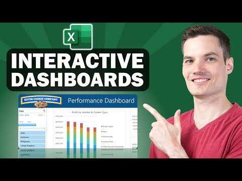
📊 How to Build Excel Interactive Dashboards
 0:13:53
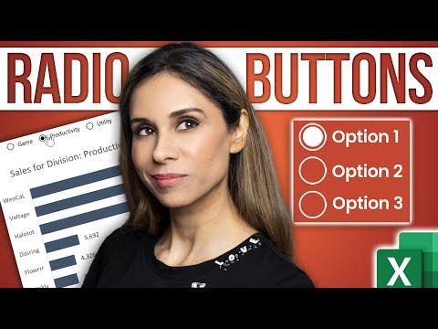
Create INTERACTIVE Excel Dashboards With Option Buttons | How to use Radio Buttons
 0:03:29
Interactive Charts in Canva
 0:09:44
How To Create Charts & Graphs in Canva
 0:00:22
Easy AI Tool for Charts and Graphs 📊
 0:00:51
Fun PIE CHARTS in PowerPoint #Powerpoint #tutorial
 0:11:54
How to create Interactive PowerPoint Charts the easy way
 0:08:22
Scrolling table | Chart | Google Sheets
 0:06:47
Analyzing And Creating Interactive Charts Directly From Microsoft Word
 0:10:15
Effortlessly Create Dynamic Charts in Excel: New Feature Alert!
 0:09:12
Build interactive charts with Form Controls
 0:12:53
🌍 How to make interactive Excel Map charts
 0:15:18
Interactive Charts with Reaction Labels- Impress Your Boss
 0:02:38
How to Create Interactive Charts with Checkboxes in Excel
 0:10:42
How to create Interactive Charts in Microsoft Excel using Data Validation List
 0:04:40
How to Create Interactive Charts from Excel Data - Five Minute Python Scripts
 0:08:09
Excel Dynamic Chart with Drop down List (column graph with average line)
 0:12:39
Smart Excel Pivot Table Trick - Choose Your KPI from Slicer (Excel Dashboard with DAX)
 0:00:26
How to create Map Charts in Excel? | Excel Tricks #shorts #excel
 0:00:56
Don't Create Charts Manually in Power BI‼️Instead Use AI Feature😎 #powerbi #chart #shorts #exce...
 0:06:33
How to Create Interactive Charts and Diagrams in Google Slides
 0:14:48
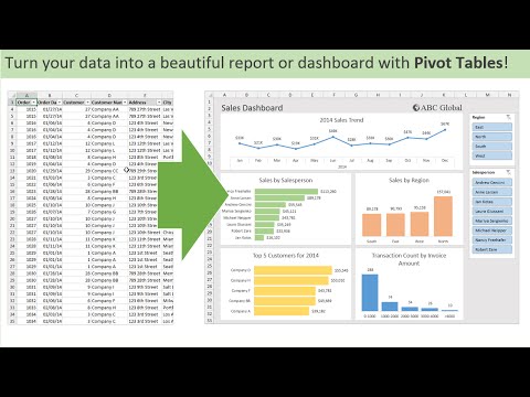
Introduction to Pivot Tables, Charts, and Dashboards in Excel (Part 1)
 0:00:55
Google Sheets | Scrolling table to your Dashboard #googlesheets #tutorial #charts #spreadsheet
Комментарии