filmov
tv
Standard edgeR Workflow: edgeR Video Tutorial 1

Показать описание
 0:21:59
Standard edgeR Workflow: edgeR Video Tutorial 1
 0:32:44
Intro to Bioinformatics - EdgeR pt 1 - VDB Computational Biology
 0:17:13
Intro to Bioinformatics - EdgeR vs DESeq2 - VDB Computational Biology
 0:30:36
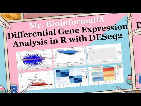
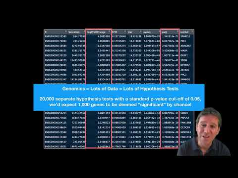
Differential Gene Expression Analysis in R with DESeq2| Bioinformatics Tutorial for Beginners
 0:21:58
Multifactor Designs in DESeq2
 0:12:10
Differential Expression for RNA-Seq Part 1: Using the limma Bioconductor package
 0:26:33
Differential expression analysis
 0:01:58
deseq tutorial & visualization. how to plot dispersion estimates
 0:19:46
DESeq2 workflow tutorial | Differential Gene Expression Analysis | Bioinformatics 101
 0:25:32
DESeq2 Basics Explained | Differential Gene Expression Analysis | Bioinformatics 101
 0:00:23
How to install tile edge trim(4 steps)
 0:14:56
9.2 Differential expression tests and pathway analysis
 0:25:20
STAT115 Chapter 5.2 Differential RNA-seq
 0:56:18
The Magic of Multifactor Testing
 0:27:00
How Does DESeq2 Work?|Bioinformatics for Beginners|Differential Expression Analysis|Mr BioinformatiX
 2:43:03
Tidy Transcriptomics
 0:53:07
Stefano Mangiola, Maria Doyle, Workshop 100: A tidy transcriptomics introduction to RNA Seq analyses
 0:57:43
Expression and Differential Expression
 0:09:56
Differential Expression Analysis with DESeq2
 0:01:39
Differential Gene Expression: Bulk RNA Seq with DESEQ2 on the T-BioInfo Platform (Getting Started)
 0:09:52
How to use Hyperledger Fabric chaincode events with cc-tools
 0:27:39
RNA-seq course: Alignment using TopHat (old)
 0:33:13
11 Apr 2019: 'Pachyderm': John Karabaic
 0:13:36
B4B: Module 2 - RNAseq analysis workflow
Комментарии