Python Tutorial: Simple Linear Regressions

---

In this video, you'll learn about simple linear regressions of time series.

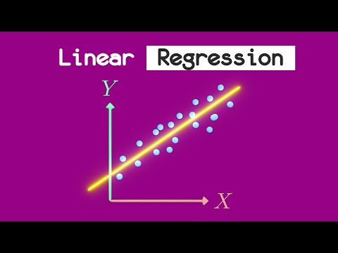
A simple linear regression finds the slope, beta, and intercept, alpha, of a line that's the best fit between a dependent variable, y, and an independent variable, x. The x's and y's can be a two-time series.

A linear regression is also known as Ordinary Least Squares, or OLS, because it minimizes the sum of the squared distances between the data points and the regression line.

Regression techniques are very common, and therefore there are many packages in Python that can be used. In statsmodels, there is OLS. In numpy, there is polyfit, and if you set degree equals 1, it fits the data to a line, which is a linear regression. Pandas has an ols method, and scipy has a linear regression function. Beware that the order of x and y is not consistent across packages.
All these packages are very similar, and in this course, you will use the statsmodels OLS.

Now you'll regress the returns of the small cap stocks on the returns of large cap stocks. Compute returns from prices using the "pct_change" method in pandas. You need to add a column of ones as a dependent, right-hand side variable. The reason you have to do this is because the regression function assumes that if there is no constant column, then you want to run the regression without an intercept. By adding a column of ones, statsmodels will compute the regression coefficient of that column as well, which can be interpreted as the intercept of the line. The statsmodels method "add constant" is a simple way to add a constant.

Notice that the first row of the return series is NaN. Each return is computed from two prices, so there is one less return than price. To delete the first row of NaN's, use the pandas method "dropna". You're finally ready to run the regression. The first argument of the statsmodel regression is the series that represents the dependent variable, y, and the next argument contains the independent variable or variables. In this case, the dependent variable is the R2000 returns and the independent variables are the constant and SPX returns. The method "fit" runs the regression and results are saved in a class instance called results.

The summary method of results shows the entire regression output. We will only focus on a few items of the regression results. In the red box, the coefficent 1-point-1412 is the slope of the regression, which is also referred to as beta. The coefficient above that is the intercept, which is very close to zero. You can also pull out individual items from results, like the intercept, in results-dot-params zero, and the slope, in results-dot-params one.

Another statistic to take note of is the R-Squared of 0-point-753. That will be discussed next.

From the scatter diagrams, you saw that the correlation measures how closely the data are clustered along a line. The R-squared also measures how well the linear regression line fits the data. So as you would expect, there is a relationship between correlation and R-squared. The magnitude of the correlation is the square root of the R-squared. And the sign of the correlation is the sign of the slope of the regression line. If the regression line is positively sloped, the correlation is positive and if the regression line is negatively sloped, the correlation is negative. In the example you just analyzed, of large cap and small cap stocks, the R-Squared was 0-point-753, the slope of the regression was positive, so the correlation is then positive the square root of 0-point-753, or 0-point-868, which can be verified by computing the correlation directly.

Now it's your turn.