Metavisual Geometry and Urban Economics: Detroit Example Pt 1

This preliminary analysis technique provides us with a "rough draft" of land values, population density, and building height. It gives us a place to start in order to delve deeper into a more detailed analysis. Detroit (Cite De Troit--City of the Strait), Michigan, USA and the surrounding region has roots of in a civilization that dates back to at least 500 BCE. Similar to Alaise, Detroit has a series of radial paths.
I began this project in the 1980s and turned a simpler version into my doctoral dissertation (reshaped into Agglomerative Subcenters: In Monocentric Cities, ISBN-13: 978-1491061169). Though the principles remain the same, I have been able to take it much deeper. In addition, this process of modeling is applicable to ancient sites such as Alaise and similar earlier civilizations. I hope that you enjoy this short overview that I have prepared as an introductory tutorial for students of all ages.

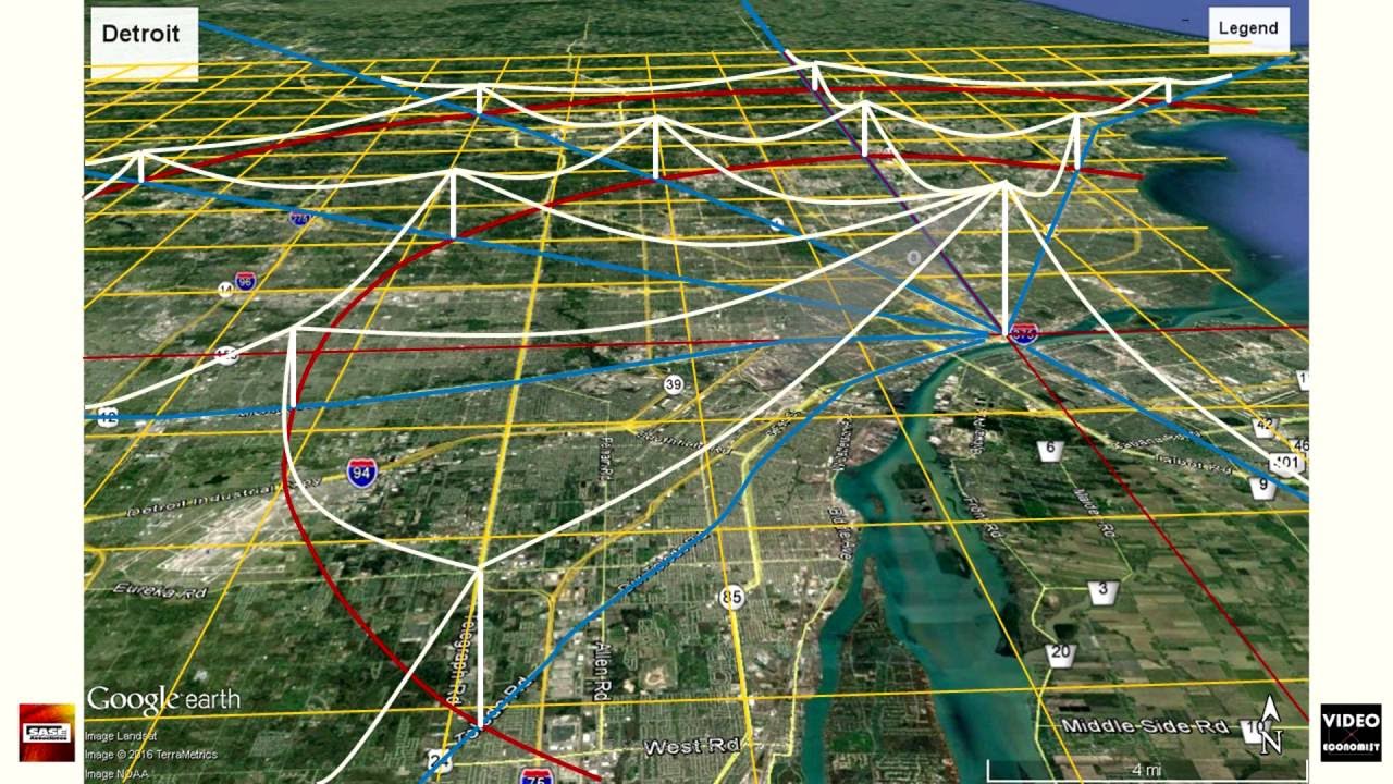
1. We start with a northward perspective of Detroit,
2. extending lines from the Central Business District,
3. and creating a grid with longitudes and latitudes placed every four miles to form squares of sixteen square-miles. Given the township survey and layout of state roads in Michigan, this pattern is convenient for further subdivision.
4. We highlight the CBD coordinates in red
5. and place markers on these lines at 17 miles from the CBD. Using this Cartesian Plane, we locate other points of the same radial distance at points on the grid.
6. We identify them by setting 17 miles squared equal to the sum of longitude miles squared and latitude miles squared.
7. Next, we add the ancient primary paths known today as Michigan, Grand River, Woodward, Mound Road, and Gratiot Avenues.
8. We locate coordinates for a
9. secondary ring at a radial distance of 32 miles.
10. Let’s reduce the brightness of the principal radial paths
11. and extend the grid in the southeast.
12. We also extend the Woodward path into Windsor, Ontario, Canada.
13. Then, we draw the Southwest path known as the Toledo Road.
14. Building our model, we add vertical density-axes at the CBD and at points along the radial paths intersecting with the subcenter rings. With these axes, we can measure the density of land values, population, or building height. Depending on the density to be measured, we scale them to the appropriate units. Wishing to vary the relative height of these vertical lines, we mark the CBD
15. as the tallest with an Index value of One.
16. For the first ring of subcenters, let’s reduce the height Index of the vertical axes to 50% while
17. decreasing this Index at the outer-ring subcenters to 25%.
18. Next ,we add density curves between local maximum points.
19. With actual data, these curves can be estimated using U-shaped quadratic and asymptotic negative-exponential functions. These functions can be integrated both radially and laterally.
20. Using similar lines,
21. the secondary lateral curves are wider and lower than the first.
22. Finally, we complete our topological surface of densities by taking the double integral of the sum of all functions combined. This combination of topological algebra and integral calculus produces a density surface that resembles the sheeting of a circus tent. Our system remains flexible by allowing us to add or delete subcenter axes, vary their height, and otherwise alter our model as needed.