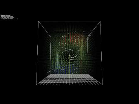
Stable Fluids implemented in Python/NumPy

Unconditionally stable means that the time steps can be chosen arbitrarily large, and the kinematic viscosity can also be selected freely. This is extremely advantageous for computer graphics applications. Surely, this algorithm is unable to compete with state-of-the-art CFD codes in terms of accuracy and modelling capabilities. However, I think it is beautiful and encourages one to dig deeper.

-------

-------

Timestamps:
00:00 Introduction
00:23 About Stable Fluids
00:59 Problem Scenario
01:14 Upwards Forcing
01:31 Algorithm in Detail
04:06 Note on Boundary Conditions
04:17 Imports
05:11 Defining Simulation Parameters (=Constants)
05:53 Some Boilerplate
06:07 Creating a mesh
09:24 Forcing Function Definition
11:39 Vectorizing the Forcing Function
12:33 Time Loop + Initial condition
13:09 Step 1: Apply forces
13:50 Step 2: Nonlinear Convection (Self-Advection)
17:04 Step 3: Diffuse
17:19 Laplace Operator
18:58 Implicit Diffusion Operator
20:46 Step 3: Diffuse (cont.)
22:30 Step 4.1: Compute Pressure
23:00 Divergence + Partial Derivatives
26:00 Poisson Operator
26:54 Step 4.1: Compute Pressure (cont.)
27:53 Step 4.2: Pressure Correction
28:07 Gradient Operator
29:31 Step 4.2: Pressure Correction (cont.)
30:04 Advance in time
30:22 Initial visualization
31:43 First run + debugging
32:47 Curl Operator
34:00 Visualizing the Curl
36:15 Discussing the Plot
36:51 Playing with the Viscosity
37:20 Instability
37:56 Outro

[programming]

I was expecting this to have so many more views. Great job!

[fexvfx]

Ich finds geil wie du from scratch das einf mal so dahincodest und dabei super erklärst 😅

[Anzo]

Thank you for making this excellent video and the impressive, efficient implementation! I have a question though regarding the diffusion operator which I might have misunderstood. Should the diffusion operator not be the discretised form of A = [ identity - viscosity * dt * \nabla^2 ] which is solved for with b = the advected vector field (w_2 in Stam's paper) as part of the linear system? In your code, A seems to be already premultiplied by the advected vector field (w_2) which is only meant to be b in the linear system.

[RedTiger]

Just curious with the partial derivative x function, in the python code, it seems doing the subtraction along the y direction. so is the partial derivative y function, Is it a fault ?

[achalpandeyy]

Hi, I have a question.
After the step 4.2 "Correct the velocities to be incompressible", when I compute the divergence (with the same function as defined in the code) of `velocities_projected` I still get non-zero divergence values. Why is that? Isn't making the divergence 0 the entire reason we did this step?

[heavennoes]

I tried this code on Jupiter but it is showing per 'frame'

[maximegr]

Hello man, really liked the video. I am trying to use the same algorithm for other configurations but I need to implement boundary conditions. Any idea on how to do this ? Thanks in advance

[sudeephalder]

Can you please tell me in detailed that how you are creating the animation of this fluid flow??? I can plot, but not able to animate. Kindly help

[Kaassap]

great video! Is there a reason for not using object oriented programming?

[jhanolaer]

Sir, just asking.. how do i combine or interact the density arrays and velocity arrays?

[snusnufreak]

This looks very similar to the finite difference approach you used to solve the open-lid problem in another of your videos. I wish I could learn the subtleties, where would you suggest to start?

[brtw]

Hey man! Do you have any platform in which I could message you on? /an email I could send to, have an enquiry!