filmov
tv
Simple Linear Regression in NCSS

Показать описание
In this video tutorial, we'll cover the basics of performing a Simple Linear Regression analysis in NCSS.
Simple Linear Regression is a method for studying the relationship between a dependent variable, Y, and a single numeric independent variable, X. Simply put, linear regression is used to estimate the intercept and slope of the straight line that give the best fit to the observed data. This line, called the least squares regression line, can be used to describe the relationship between the two variables or to predict Y at given values of X.
For our example, we'll use a small dataset that contains measurements of X and Y from 25 subjects and perform a very basic simple linear regression analysis.
With the dataset loaded, open the Simple Linear Regression procedure using the menu. Click Reset to load the procedure with the default settings.
On the variables tab, enter Y as the dependent variable and X as the independent variable. If we were to enter several Y variables, then a separate analysis would be performed for each variable.
On the reports tab, we'll deselect everything except the Run Summary, Regression Estimation, and Assumptions reports since these are the reports we'll focus on.
On the plots tab, let's deselect the histogram, again to reduce the size of the output, and also add confidence limit lines to the probability plot. The plots will help us to check the critical assumptions for this analysis.
Click Run to perform the analysis and generate the report.
First, look at the Y versus X scatterplot and decide if a straight line really fits the data. In this case, the line looks like it fits the data pretty well. The R-squared value of 0.959, given in the Run Summary Report, indicates a pretty good fit. The closer the R-squared value is to one, the better the fit.
If the results had appeared like they do in this other plot, however, we would conclude that a straight line does not fit the data well at all and that simple linear regression should not be used. One solution would be to transform Y by taking the logarithm or square root so that the relationship is linear. A better alternative, however, would be to fit a curved line, like the one here in blue. NCSS provides many additional nonlinear regression and curve fitting tools for fitting curved lines to this type of data.
Another basic assumption in linear regression is that the variance of the residuals is constant over the range of the X's. We can check this assumption using the Residuals of Y versus X plot. Here we are looking for a constant, rectangular scatter in the residuals over the entire range of X. In this case, the assumption appears to be met. The Levene test from the numeric portion of the report further supports our conclusion that this condition is met.
In contrast, if the residual plot had looked as it does here with a Megaphone- or V-shaped residual scatter, or as it does in this plot with a clearly identifiable pattern then we would have to conclude that the constant-variance assumption is violated. We could try applying a variance-stabilizing transformation by taking the logarithm or square root of Y and then re-running the analysis with the transformed data.
Finally, we can look at the Normal Probability Plot to determine if the assumption that the residuals are normally distributed is satisfied. The points on the probability plot should be relatively close to the normal line and within the confidence limits, which appears to be the case here. Additional numeric tests of residual normality support the conclusion that this assumption is valid.
A probability plot like the one seen here, however, indicates departure from normality in the lower tail of the distribution. The points trail off in the lower portion, with some of them outside of the confidence limits. Again, a transformation on Y might be in order to correct the problem.
Now that we have determined that the assumptions for simple linear regression are met, we can proceed to interpret the results.
The Regression Estimation Section presents the intercept and slope estimates for the regression line. A p-value of 0.000 for the t-test of the slope indicates that the slope is significantly different from zero and that there is a relationship between X and Y. The fitted equation states that for every one unit increase in X, the value of Y goes up by 5.075 units. If we were to plug in a value for X, the equation would tell us what value to expect for Y. For example, the predicted value of Y if X is 70 would be 182.3988.
This equation, though, is really only valid over the range of X in the data! We should use caution when extrapolating these results to values of X which are less than 50 or greater than 80.
We hope that you have found this tutorial helpful. For more information about Linear Regression in NCSS or any of the other procedures, please see the Help documentation that is installed with the software.
 0:05:54
 0:09:45
 0:03:47
 0:47:34
 0:06:25
 0:06:08
 0:03:48
 1:02:14
 0:06:04
 0:02:24
 0:04:11
 0:02:11
 0:02:05
 0:00:27
 0:03:16
 0:04:14
 0:08:15
 0:28:50
 0:04:49
 0:07:02
 0:03:08
 0:03:46
 0:04:42
 0:02:59