Financial Mathematics for Actuarial Science, Lecture 1, Interest Measurement

Begin your journey toward a career in finance or as an actuary! This lecture introduces the foundational concepts of the theory of interest: the time value of money, simple interest, compound interest, and various ways of mathematically representing compound interest. This content is essential if you want to understand annuities and bond markets.

(0:00) Introduction and textbook.
(1:48) The time value of money (most people would prefer $1 right now than one year from now).
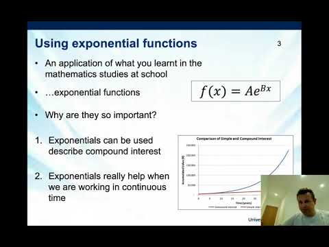
(3:35) Simple interest and compound interest formulas, both for the interest earned and the accumulated amount (future value).
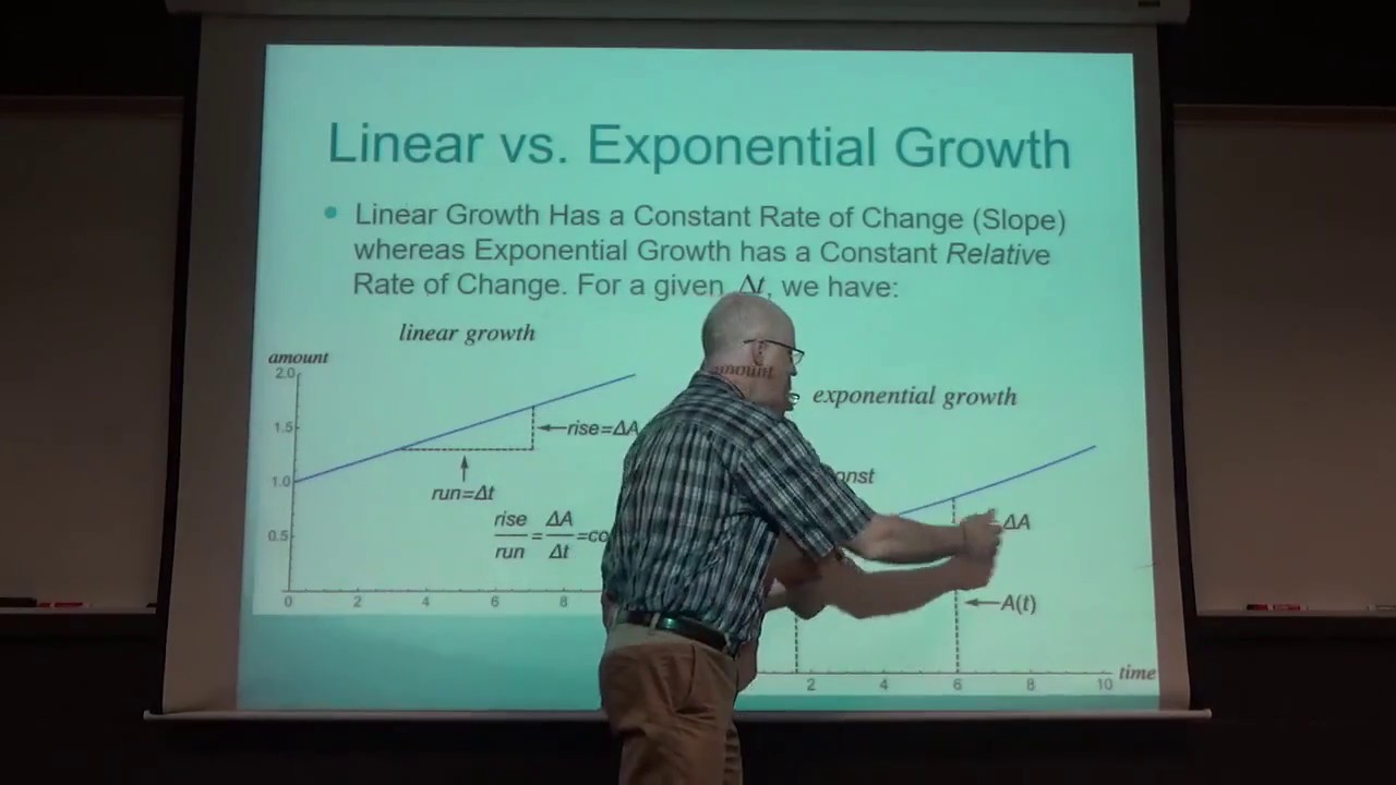
(4:52) Linear growth versus exponential growth. Linear growth has a constant rate of change: the slope is constant and the graph is straight. Exponential growth has a constant relative rate of change (percent rate of change). Mathematica animation.
(8:27) Actuarial notation for compound interest, based on the nominal interest rate compounded a certain number of times per year.
(11:38) The graph of the accumulation function a(t) is technically constant, because banks typically make discrete payments of interest.
(12:34) It's very important to make timelines to help you solve problems (time diagrams).
(15:46) Relating equivalent rates (when compounding occurs at different frequencies) and the effective annual interest rate.
(18:37) Continuously compounded interest and the force of interest, which measures the constant instantaneous relative rate of change. Given the force of interest, you can also recover the amount function a(t) by integration.
(26:04) An odd-ball example where the force of interest is sinusoidal with a period of 1.
(30:08) Present value basic idea: how much should you deposit now to grow to A after t years? (32:48) Present value discount factor. For a constant value of i, it is v = 1/(1+i) = (1+i)^(-1). Example when i = 0.10. Also think about timelines and pulling amounts back in time.
(37:43) Present value for a varying force of interest and the odd-ball example.
(41:40) The present value discount rate d = i/(1+i) = 1 - v (percent rate of growth relative to the ending amount). Bond rates are often sold at a discount. Other relationships worth knowing. The ID equation i - d = id.
(45:30) Equivalent ways of representing the accumulation function a(t) and its reciprocal. (46:45) Inflation and the real interest rate. The real rate is (i - r)/(i + r).

Overall Video Topic: Financial Quantities Representing Growth and Decay (especially exponential).

Bill Kinney, Professor of Mathematics at Bethel University in St. Paul, MN.

Bill Kinney Math.

AMAZON ASSOCIATE
As an Amazon Associate I earn from qualifying purchases.

[jared]

The amount of time and effort you must put into teaching at your university PLUS Youtube is incredible... thank you Prof Kinney for going above and beyond so that we can learn at our own pace and make sure what we're doing is right!

[lukealadeen]

People like Bill Kinney, that impart knowledge to people all over the world, without demanding anything back, exemplify the greatest attributes of human beings. Thank you Sir.

[crabfood]

I’m a freshmen in high school and i LOVE math and I have been considering of being an actuary so I try to learn things as early as possible to have a little head start. It may be a bit too early but I wanna see what i’m getting myself into so I can have an idea of what I really want to be in the future. Thank you for making this ! :)

[Pabloescobar]

Prof Kinney your amazing, thank you so much for taking the time to go in depth and help us learn at our own pace. Unfortunately my prof makes us teach ourselves so this has been a life saver!

[ofyourbluesky]

Bill, you knocked it out of the park. FANTASTIC job!

[FiorianCanuck]

Thank you Prof Kinney! Amazing work and very informative!

[jayeshmanghani]

I really appreciate your effort Professor...
Thank you very much sir... Please keep making videos and let mathematics be alive forever...

[lakshayguglani]

Thank You Sir for putting together such a great tutorial.

[junal]

excellent video, how oppotune the last discussion regarding inflation, if you push forward your 2017 discussion to today's Augus thanks you teacher, your videos are helping me to prepare the SOA FM

[mikehipparchusnewton]

e is definitely the most interesting transcendental number i.m.o.

[ify]

The moving animation of the slope helped a lot to understand

[jacobm]

Are these lectures comprehensive? Meaning these are all the material covered for the exam? love the videos!

[svobodaalexendra]

Hi Bill, thanks for uploading great video! I am working in data analytics industry and recently I found that actuary is very interesting but don't know where to start from. Currently I am doing self-study using videos on YouTube (probabilities, Actuarial sciencelectures etc), but not sure whether this would be enough to be an actuarial analyst.

[absidyabsidy]

Hey, would this lecture series (along with your problem-solving videos) cover all/most of the content necessary for the FM actuarial exam? If not, what resources do you recommend getting my hands on? I have a strong math background.

[jared]

35:07 did you mean to say "the PV of an amount of 1, one year in the future, is 90.9% of what it is (91 cents or .91 dollars) at time zero - instead of ".91cents if you will at time zero"

[raspberryheaven]

Is there any book you can recommend to accompany this lecture?

Btw, thank you sir!! 😊

[naveenamarendra]

28:34 can someone explain how they got 11.22% as the effective annual interest rate

[ved]

I'm currently pursuing a bachelor's in engineering and am interested in starting off with the exams for the iFoa . Is it better to start clearing exams and working or Working towards getting a master's in actuarial science?

[lenonngomana]

What mathematical knowledge do we need for this course

[davidgerardstack]

love the lectures - suggest the oddball example is not useful