Python Tutorial: Calculate cohort metrics

---

Great! We have assigned the cohorts and calculated the monthly offset for the metrics. Now we will learn how to calculate business metrics for these customer cohorts. We will start by using the cohort counts table from our previous lesson to calculate customer retention. Then we will calculate the average purchase quantity.

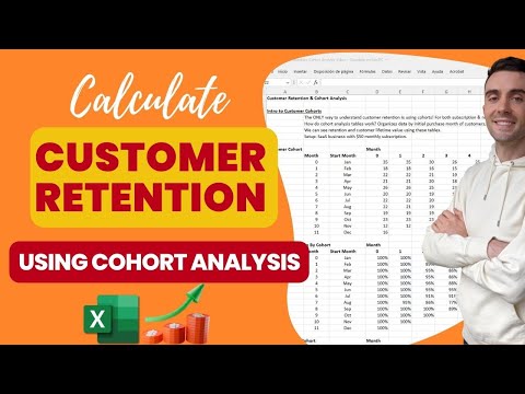
The retention measures how many customers from each of the cohort have returned in the subsequent months.

We will use the dataframe called cohort_counts which we created in the previous lesson. Our first step is to select the first column which is the total number of customers in the cohort.

Next, we will calculate the ratio of how many of these customers came back in the subsequent months which is the retention rate.

One word of caution, you will see that the first month's retention - by definition - will be 100% for all cohorts. This is because the number of active customers in the first month is actually the size of the cohort.

We will select the first column from the table and store it as cohort_sizes.

Then we will use the divide() function on the cohort_counts dataframe and pass the cohort_sizes. We set the axis parameter to zero to ensure we divide along the row axis.

Finally, we round the ratio to 3 digits and multiply it by a 100 to make it look like a percentage.

With these simple commands, we have completed retention metric calculation. Let's take a look at it.

As you can see, the first column has a 100% retention rate for all cohorts, as expected. We can now compare the retention rate over time and across cohorts to evaluate the health of our customers' shopping habits.

Let's take a look at another example.

Let's step back a little bit and go back to our original online dataset. We will show you how to calculate other metrics for these cohorts.

These are almost identical lines of code you've seen in the previous slide where we created the customer_counts. What's different is that in this case, we will calculate the average quantity.

First, we create a groupby() object with CohortMonth and CohortIndex and store it as grouping.

Then, we call this object, select the Quantity column and calculate the average. Then we store the results as cohort_data.

Then, we reset the index before calling the pivot function to be able to access the columns now stored as indices.

Finally, we create a pivot table by passing CohortMonth to the index parameter, CohortIndex to the columns parameter, and the Quantity to the values parameter.

Let's round it up to 1 digit, and see what we get.

Here we go! You are now fully equipped to manipulate transactional customer data and draw powerful insights.

Now you will practice what you've learned so far and will build new analyses with additional metrics!