Data Visualization using python libraries | matplotlib I Seaborn | plotly with examples

Visualization is any technique for creating images, diagrams, or animations to communicate a message.
Types of Data Visualizations :
Explanatory:
Exploratory:
#jaganinfo
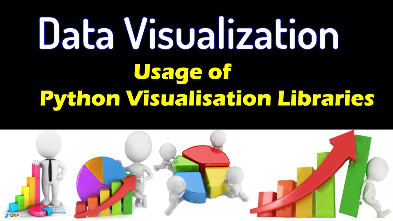
Python Visualisation Libraries
• Matplotlib
• Pandas built-in plotting
• ggpy
• Altair
• Seaborn
• Plotly
• Bokeh
• HoloViews
• VisPy
• Lightning
 
Visualization methods :
Distribution
It is commonly used at the initial stage of data exploration i.e. when we get started with understanding the variable. Variables are of two types: Continuous and Categorical. For continuous variable, we look at the center, spread, outlier. For categorical variable we look at frequency table.
Histogram : It is used for showing the distribution of continuous variables.
Box-Plot : It is used to display full range of variation from min to max and useful to identify outlier values.
Comparison
It is used to compare values across different categories.
Common charts to represent these information are Bar and Line chart.
Bar Chart : It is used to compare values across different categories
Line Chart : It is used to compare values over quantitative variable
Composition
It is used to show distribution of a variable across categories of another variable
Pie Chart : It can be created by passing the values representing each of the slices of the pie.
Relationship
It is widely used to understand the correlation between two or more continuous variables
Scatter Plot : It clearly shows the relationship between two variables

Demo 1 : Basic Plot

Demo 2 : Basic Plot Legend Title Labels
x,y = [1,2,4],[5,7,4]
x2,y2 = [1,2,5],[8,11,5]

Demo 3 : Bar Chart
x = [2,4,6,8,10]
y = [6,7,8,2,4]
x2 = [1,3,5,7,9]
y2 = [7,8,2,4,2]

Demo 4 : Hist Chart
population_ages = [22,55,62,45,21,22,34,42,42,4,99,102,110,120,122,130,111,151,115,112,80,75,65,54,44,42,48]
bins = [0,10,20,30,40,50,60,70,80,90,100,120]

Demo 5 : Scatter Plot
x = [1,2,3,4,5,6,7,8]
y = [5,2,4,2,1,4,5,2]
# google matplotlib marker option

Demo 6 : Stack Plot
days = [1,2,3,4,5]
sleeping = [7,8,6,11,7]
eating = [2,3,4,3,2]
working = [7,8,7,2,2]
playing = [8,5,7,8,13]

Demo 7 : Pie Charts
days = [1,2,3,4,5]
sleeping = [7,8,6,11,7]
eating = [2,3,4,3,2]
working = [7,8,7,2,2]
playing = [8,5,7,8,13]
slices = [7,2,2,13]
activities = ['sleeping','eating','working','playing']
cols = ['m','c','r','g']
# startangle , shadow= , explode , autopct

Demo 8 : Load Data from Files
import numpy as np

Demo 9 : Live Graphs
from matplotlib import style
def animate(i):
xaxis = []
yaxis = []
for line in lines:
if len(line) greaterthan 1:
ani = animation.FuncAnimation(fig, animate, interval=1000)