filmov
tv
2. Preferences and Utility Functions

Показать описание
MIT 14.01 Principles of Microeconomics, Fall 2018
Instructor: Prof. Jonathan Gruber
This video focuses on the demand curve, derived from how consumers make choices, and the supply curve, which is how firms make production decisions.
Chapters
00:00 Title slate
00:11 Lecture Start
01:13 Model Assumptions
05:54 Indifference Curves
09:23 Four Properties
13:27 Real Example ( job search )
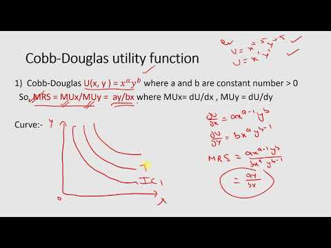
15:28 Utility Functions
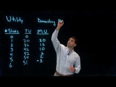
18:31 Margin Utility
24:49 Marginal Rate of Substitution
30:13 Why graph's not concave
32:37 (Q) Addictives & MRS
34:31 Price of Different Sizes of Goods
License: Creative Commons BY-NC-SA
Instructor: Prof. Jonathan Gruber
This video focuses on the demand curve, derived from how consumers make choices, and the supply curve, which is how firms make production decisions.
Chapters
00:00 Title slate
00:11 Lecture Start
01:13 Model Assumptions
05:54 Indifference Curves
09:23 Four Properties
13:27 Real Example ( job search )
15:28 Utility Functions
18:31 Margin Utility
24:49 Marginal Rate of Substitution
30:13 Why graph's not concave
32:37 (Q) Addictives & MRS
34:31 Price of Different Sizes of Goods
License: Creative Commons BY-NC-SA
 0:41:24
2. Preferences and Utility Functions
 0:43:40
Preferences and Utility Functions 2 Indifference Curves
 0:10:52
Indifference curves and marginal rate of substitution | Microeconomics | Khan Academy
 0:04:47
Preferences relation from utility function
 0:06:48
UTILITY FUNCTION ( 4 types)I MICROECONOMICS
 0:21:13
Managerial Economics 3.1: Preferences and Utility
 0:05:49
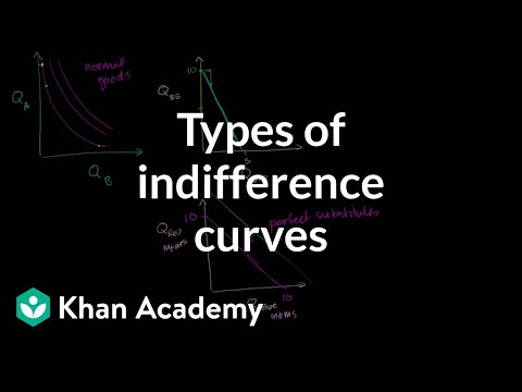
Types of indifference curves | Microeconomics | Khan Academy
 0:05:41
1.5 Utility Functions
 0:11:42
Preferences| Strict & Weak Preference| Varian Ch 3| BA (H) Economics| NTA NET Economics| IES |
 0:50:40
Preferences and Utility Functions 1
 0:08:28
Indifference Curves
 0:10:13
Utility Theory - Total, Marginal and Average Utility
 0:06:58
Utility function when goods are perfect complements
 0:04:43
Different utility functions may represent the same preferences
 0:27:32
Lecture 44(A): Representation of Preferences by Utility Functions
 0:32:49
Intermediate Microeconomics: Utility (Lecture 4)
 0:12:31
Utility & Marginal Utility
![(M3E6) [Microeconomics] Utility](https://i.ytimg.com/vi/Alu1DCMiTD4/hqdefault.jpg) 0:07:23
0:07:23
(M3E6) [Microeconomics] Utility Maximization Problem with Quasi-Linear Utility Functions
 0:03:51
Utility function
 0:14:20
Introduction to Utility Functions
 0:05:41
Homothetic Utility Functions and Preferences
 0:11:02
Micro: Unit 2.2 -- Utility Maximization
 0:04:35
Utility Functions: Positive Monotonic Transformations
 1:30:35
Chapter 21: Theory of Consumer Choice - Utility Maximization
Комментарии