Highlight Cells that Match with Conditional Formatting

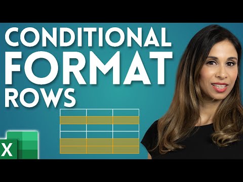
Say you have a table of records and you wanted to show where there were matches to a value. You could use the find function to do this but what if you wanted to have it show more? Like have it highlighted in a color? There is a way to do this and it's with the Conditional Formatting feature in Excel. You input a value somewhere and Excel will search for it in your table and highlight the rows that have that value. I'll show you a way to do this with as using a case sensitive (matching upper case or lowercase) and case in-sensitive match. See the video to learn how.

📝 This description may contain affiliate links and we'll receive a small commission if a purchased is made using the links (but at no additional cost to you). It'll support the channel and so more videos like this can be made. Thanks for your support!

#excel
#msexcel
#doughexcel

-~-~~-~~~-~~-~-
Please watch: "Convert Table in a PDF File to Excel"
-~-~~-~~~-~~-~-

[nalcantara]

Thank you! Exactly what I was looking for.

[pauloyvens]

Simple but very usefull... thank you Doug

[bluffmasterhara]

Thanks Doug! This is the 2nd time you've really helped me

[bartholomewallen]

THANK YOU SO MUCH! I had to generate a report with this functionality and works as expected.

[JayJaeRockCity]

Hey cool.... USVI in the House!!! Got excited when I saw that. Let me finish the video.

[biankastubblefield]

Hey U.S Virgin Islands! That's where I'm from! Thanks for the help

[diensamaniego]

Hi! This was really helpful. I already did what you taught in the video but is there a way where the highlighted cell will not be replaced once you change then details on the Enter SKU? That would be really helpful! Thank you

[usamamando]

Can we change the formatting (e.g. color) of some arbitrarily selected cells of a table in Word using a selection of combo box or dropdown list content control so that only the cells of the selected selection are formatted (active)... one color enough...

[wulfrum]

What if I wanted to highlight from a list and not just two items? Let's say I have 100 items in List A, and I want List B (containing 30 items) to be highlighted in List A?

[izygh]

How can you use the ''equal to'' preset conditional formatting in excel to format multiple values in a range at once and not one at a time? Or if there is a better alternative to this conditional formatting, what is it, please?

[tazrianalamjitu]

How can I get all highlighted cell display together in top of the table!?! Please let me know if you can.
Thanks in advance

[scorchpunyasubhan]

how, if 3 column (a5=contain text "right";b5.f5=contain text "o"), the row will changed color to green and text to white

[jerryfriday]

Good day,
I must admit it is a gift to stumble on this article, but however my challenges was not addressed. I have a work sheet with just a single column. I need a formula that will highlight the row above the cell if the cell contains a specific text. For example if A2 contains "great" A1 should be highlighted. Thank you so much while i await your response.

[luminkyaw]

This is really helpful and thank you so much. Btw how do I make connection between these two data, means, if I select colour in format for all data and the same colour is showing in "QEWR65UYE" that u used in this example?

[TODOMATIO]

I only want to highlight duplicate cells in FILTERED rows, only in selected rows. Instead it’s highlighted everything because it’s checking all the table. Of course all will be duplicate if you check the whole table. I need to see unique numbers in my filtered results

[StormyTsormy]

I need to highlight cell having two matching strings. AND condition. How do I do it?

[investmentnre-pwc]

but that is cannot used in merge cells

[georgebanin]

Can I conditional format data I haven't yet entered

[NaZReD]

is there away to display the scores flipped? so, F2 = F2, F3 = G2, F4 = H2, i.e. the names across the top and the scores display downwards? i been trying to flip the codes but keep getting errors thank you,

[jayephgee]

THIS DOES NOT WORK!

I am trying to format a formula where a cell is highlighted if it matches the value based on another cell. For some DUMB REASON, when I enter the formula I am using into a blank column, it returns FALSE, which it's NOT FALSE! The formula that I am using for the condt'l format is: "=$E3=$A$2" and when I press Enter, IT DOESN'T FORMAT IT CUZ THE LOGICAL RESULT IS FALSE WHEN IT SHOULDN'T BE!

What am I doing wrong??