Kalman Filter for Beginners, Part 2 - Estimation and Prediction Process & MATLAB Example

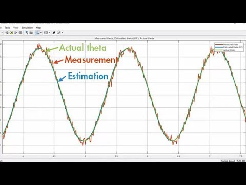
Use the Kalman Filter, even without knowing all the theory! In Part 2 of my three-part series, I discuss the prediction and estimation processes, making an analogy with low-pass filters. We construct a system model via the state transition matrix A, the state-to-measurement matrix H, and the process noise and measurement noise matrices, Q and R.

This special lecture series takes us into *dynamic* attitude estimation, using time-varying gyroscope data, as opposed to the previously covered *static* attitude estimation, which uses simultaneous measurements of known external objects.

► Next: Kalman Filter for Beginners, Part 3- Attitude Estimation, Gyro, Accelerometer, Velocity via Position

► Previous, Kalman Filter for Beginners, Part 1 - Recursive Filters & MATLAB Examples

► More lectures posted regularly

► Dr. Shane Ross 🌠 aerospace engineering professor, Virginia Tech
Background: Caltech PhD | worked at NASA/JPL & Boeing
Research website for @ProfessorRoss

► Follow me on Twitter

► Space Vehicle Dynamics course videos (playlist)

► Lecture notes for Kalman Filter series (PDF)

► MATLAB Code

► Reference
Kalman Filter for Beginners: with MATLAB Examples
by Phil Kim (Author), Lynn Huh (Translator), 2010

► Chapters
0:00 Recap
3:51 Estimation Step
8:00 Comparison with Low-Pass Filter
10:03 Error Covariance = Inaccuracy of Estimate
14:29 Prediction Step
17:34 How Prediction and Estimation Fit Together
21:44 The System Model
26:34 Covariance of the System Noise
31:30 MATLAB Simple Example
43:32 More Complicated Example

► Related Courses and Series Playlists by Dr. Ross

📚Space Vehicle Dynamics

📚3-Body Problem Orbital Dynamics Course

📚Space Manifolds

📚Lagrangian and 3D Rigid Body Dynamics

📚Nonlinear Dynamics and Chaos

📚Hamiltonian Dynamics

📚Center Manifolds, Normal Forms, and Bifurcations

Implement a Kalman filter for dummies Visually Explained tutorial MATLAB aerospace attitude estimation sensor fusion mathematics recursion orbital mechanics three body problem Lagrange Point space CR3BP 3 Manifolds James Webb Nonlinear Dynamics gravity Travel Superhighway Interplanetary Highway gravitational dynamical Astronomy astronomy wormhole physics chaos unstable Periodic Orbits Saddle Critical Halo Libration Low Energy Virginia Tech Caltech JPL Lyapunov Celestial Mechanics Hamiltonian planets moons multibody Gateway Station Lunar L1 Arches Of cislunar orbital celestial Chaotician Boeing Jet Propulsion Lab Centaurs Asteroids Comets Trojan Jupiter Family Hildas quasi Kuiper Belt

#kalmanfilter #MATLAB #lowpass #mathematics #recursion #orbitalmechanics #threebodyproblem #LagrangePoint #space #CR3BP #3body #3bodyproblem #SpaceManifolds #JamesWebb #NonlinearDynamics #gravity #SpaceTravel #SpaceManifold #DynamicalSystems #JamesWebbSpaceTelescope #solarSystem #NASA #dynamics #celestial #SpaceSuperhighway #InterplanetarySuperhighway #spaceHighway #gravitational #dynamicalAstronomy #astronomy #wormhole #physics #chaos #unstable #PeriodicOrbits #SaddlePoint #CriticalPoint #Halo #HaloOrbit #LibrationPoint #LagrangianPoint #LowEnergy #VirginiaTech #Caltech #JPL #LyapunovOrbit #CelestialMechanics #HamiltonianDynamics #planets #moons #multibody #GatewayStation #LunarGateway #L1gateway #ArchesOfChaos #cislunar #cislunarspace #orbitalDynamics #orbitalMechanics #celestialChaos #Chaotician #Boeing #JetPropulsionLab #Centaurs #Asteroids #Comets #TrojanAsteroid #Jupiter #JupiterFamily #JupiterFamilyComets #Hildas #quasiHildas #KuiperBelt

[fernandojimenezmotte]

When I first studied Linear Optimal Estimation in Advanced Control Systems [Electrical Engineering track] and in Advanced Radar Systems in Weapons System Engineering track as well, We went through all the hard derivation of the Stochastical Optimal Regulator LQR and Stochastical Optimal Estimator LQE for the whole Linear Quadratic Gaussian LQG Design for an Autopilot [in one advanced design for an American [USA] missile]. Since then Kalman have always appeared in many advanced Electrical Engineering designs. It is great to see it from the perspective of an Aerospace Engineer with scientific expertise and know how in Control and Dynamical Systems. To go very complex in advanced engineering and science doesn´t exclude any professional to get to communicate in a very didactic and understable way. You have done a great work done making Kalman Filtering, Estimation and Prediction very didatic as well as enjoyable Professor Roth. Congratulations !

[moseschuka]

Thank you so much for making this high quality tutorial available.

[johnharriott]

Best explanation of Kalman filters for new comers I have seen.

[yassiradil]

Thank you for the awesome explanation!
Never thought I'd fall in love with an algorithm😂. The stars have aligned and everything makes perfect sense now😂

[federicobusca]

This is the best series of classes I've ever seen on YT. I have my S/C Attitude Dynamics Exam in 4 days and this is so, so helpful.
Prof. Ross just made the top 5 of the teachers I've ever had in my entire school-life.
Keep up the good work!

[liku]

I am 18 years old and don't know much about these filters, and wanted to make a drone, almost everything was easy but I just couldn't grasp this concept, I think I watched more than 10 videos on kalman filter, nothing got through. But then I found this video, it was really easy to understand. thank u professor for your good work

[adamatepsilon]

coded up the Matlab example around 36:00 in python using numpy. The simple 14V is tracked really well, as in your example and the Kalman Gain and the Error Covariance decline over time. The example part is well explained and it was perfectly possible to accompish the same using python.

Then I moved on to playing around. Instead of using a constant 14V, I simulated a noisy staircase function input where voltage increases 1V every second and a sampling frequency of 1 kHz, the filter produces a ramp, not a staircase as its response is too sluggish to catch up to the new true value before it changes again. The only way to get it to perform is to set Kalman Gain to 0.1, but now I have a low-pass filter and it doesn't self-adapt anymore. (haven't seen Part 3 yet though).

EDIT: The example shown had Q set to zero. After rewatching it, I realised I had not experimented with Q. Setting Q to the standard deviation the filter started to track the noisy staircase function.

[robinamar]

Thanks a lot Prof Ross for providing a logical and simplistic explanation of Kalman Filter.
Everywhere in textbooks it is presented in a complicated manner.

[zhaoyoubing]

This video is really wonderful and helped me a lot on understanding the Kalman Filter. Thanks. Is there a small typo on 23:34 ? I think z_{k+1} on the left side of the equation should be z_{k}.

[suthakarmuthu]

Thank you for the video Professor !!! This is getting tough compare to the part1. May be i need to read it multiple times for better understanding :)

[tabhashim]

another great lecture prof. I do have a quick question however for the ending (around 48:00).
How will we actually achieve the estimation of the velocity, as the dynamic model (A matrix) just says the velocity at k+1 is equal to that of k, implying that the velocity does not change. Moreover, if we wanted to make A 3x3 and include acceleration, we would also arrive at the point where we would assume that a_k+1 = a_k (the acceleration remains constant). However, we know that neither of these two statements are true.
Where in this Kalman algorithm does it actually know how to properly update the velocity for it to actually be correct because it surely isn't coming from the A matrix?

[PannagaSudarshan]

Prof, how did you say Po- = 6 is high? @36:10 ?

[kaankutlu]

Ross thanks for your time and effort. If it is possible can you make video about how to calculate nees and nıs of Kalman filter and IMM filters

[anfarahat]

Thank you for the great explanation! What to do if we do not have a process model?

[luiggitello]

Why is it that lqe or kalman function spit out a constant gain of K without simulating the system recursively like yours?

[TheMrOlivex]

Hello Prof. Ross, thank you very much for this video series. I think you explained the Kalman Filter in a very intuitive and easy way, unlike most sources on the internet. I have one question regarding the state estimation. As far as I know you are using a state space model in the prediction step (xk = A*xk-1 +B*uk), where B*uk describes the input to the system. However you are only using the first part which describes the state transition without any input. What if your system has an input uk which you can measure. Is it then also possible to use the hole state space equation (xk = A*xk-1 +B*uk) in the prediction step?

[yyttommy]

i feel there is a gap between part 1 and part 2.

[DongGeeHong]

Wow, It's same as phil kim's book.