filmov
tv
Constrained Optimisation maximize profit function subject to constraint using Lagrange's multiplier

Показать описание
In this video we will solve a problem on constrained Optimisation.
maximise the following profit function:
π = 50x – 2x2– xy – 3y2 + 95y
St:
x + y = 25
Where x and y are the outputs of two products produced by the firm.
First we form Lagrangian function by first setting the constraint function equal to zero
25 — x — y = 0
The next step in creating the Lagrangian function is to multiply this form of the constraint function by the unknown artificial factor λ and then adding the result to the given original objective function. Thus combining the constraint and the objective function through Lagrangian multplier (λ) we have
L= 50x – 2x2 – xy – 3y2 + 95y + λ (25 — x — y)
Where L stands for the expression of Lagrangian function.
It can be seen that in this function there are three unknowns x, y and λ. Note that the solution that maximises Lagrangian function (L) will also maximise profit (λ) function:
For maximising L, we first find partial derivatives of Lwith respect to three unknown x, y and λ and then set them equal to zero. Thus
Lx = 50 – 4x – y –λ =0 …..(i)
Ly = – x – 6y + 95 — λ =0 …..(ii)
Lλ = x + y – 25 = 0 ….(iii)
Here Lx, Ly and Lλ are partial derivatives wrt x , y and λ
Note that the last equation (iii) is the constraint subject to which the original profit function has to be maximised. In fact, Lagrangian function is so constructed that the partial derivative of Lwith respect to λ (Lagrangian multiplier) always yields the original constraint function. Further, since the partial derivative of L with respect to λ is set equal to zero, it not only ensures that the constraint of the optimisation problem is fulfilled but also converts the Lagrangian function into original constrained profit maximisation problem so that the solution to both of them will yield the same result.
now, we solve the above system of three equations with three unknowns to find the optimal values of x and y by substracting the equation (ii) from equation (i)
– 45 – 3x + 5y = 0 ….(iv)
Xing equation (iii) by 3 and adding it to equation (iv) we have
– 45 – 3x + 5y =0
-75 + 3x + 3y =0/ -120 + 8y – =0
Thus, 8y = 120
y= 15
Substituting the value of y = 15 in the constraint function x + y = 25 we get x equal to 10.
The value of λ can be obtained by substituting the solved values of x and y in a partial derivative equation containing λ in the Lagrangian function. Thus, in our above example, the value of X can be obtained by substituting x = 10 and y = 15 in equation (ii) above
Thus, in the above equation (ii)
– x – 6y + 95 + λ =0
λ = x + 6y – 95
λ = 10 + 90 – 95
λ = 5
Here λ can be interpreted as marginal profit at the production level of 25 units. It shows if the firm is required to produce 24 units instead of 25 units, its profits will fall by 5. On the other hand, if firm were to produce 26 instead of 25 units, its profits will increase by about 5.
It is to be remembered that Lagrange technique maximises profits under a constraint. It does not solve unconstrained profit maximization.
This video will help you to crack any
Competitive exam for Economics like UGC NTA NET ECONOMICS, GATE ECONOMICS, UPSC , Delhi School of Economics, MA ENTRANCE ECONOMICS
JAM ECONOMICS
Check our playlist
Algebra in Economics
GATE ECONOMICS
Mathematical Economics
Integration in ECONOMICS
Matrix Algebra in Economics
GRAPHING IN ECONOMICS
Microeconomics
Comparative Statics in Economics
INPUT OUTPUT MODEL
IS-LM MODEL
You can Join
On Facebook
Facebook page
On Telegram
#MathematicalEconomics
#JAMECONOMICS
#ImportantQuestionsInEconomics
#MAEntranceEconomics
#GateEconomics
#QuantitativeEconomics
#EconMath
#GATEEconomics
#NETEconomics
#DSU
#KU
#NTA #NetEconomics #JRF #IES #Economics #MathematicalEconomics
#Economics
#Optimisation
#Constrained_Optimisation
#Gate_Economics
 0:16:07
Constrained Optimisation maximize profit function subject to constraint using Lagrange's multi...
 0:05:00
Profit maximization | APⓇ Microeconomics | Khan Academy
 0:18:09
Constrained optimization problem. find profit maximization level of output
 0:05:50
Lagrangian: Maximizing Output from CES Production Function with Cost Constraint
 0:10:17
lagrangians in economics: constrained optimization
 0:03:46
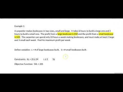
Maximizing Profit Practice
 0:15:08
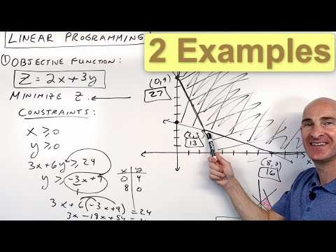
Linear Programming (Optimization) 2 Examples Minimize & Maximize
 0:10:41
Constrained Optimization. Cost minimisation from given Cost function with Production Constraint
 0:07:54
2024🎓| Ch 19 Linear Programming | Sem 3 Advanced MME | BA(H) Economics | Sydsaeter & Hammond
 0:06:29
Constrained optimization introduction
 0:14:46
Constrained Optimisation: Profit Maximisation using Excel
 0:11:37
Constrained Optimisation using Lagrange's Multiplier. #langrage #Multiplier #GATE #NET #ECONOMI...
 0:06:23
Production Function Profit Maximization Problem
 0:12:37
Maximize Profit function Subject to Constraint using Lagrange's Multiplier Example #NTA #ECONO...
 0:04:31
Constrained Revenue Maximization
 0:05:50
Profit Maximisation using Lagrange Multiplier | Constrained Optimisation
 0:15:11
constrained optimization problem. cost Minimisation
 0:17:37
Constrained optimization using Lagrange's multiplier
 0:11:02
Example 3: Finding the maximum profit (Optimization)
 0:03:45
Profit Maximization with Two Goods in Profit Function
 0:08:37
Utility Maximization using Lagrange Method. utility optimization #lagrange #utility
 0:18:03
Linear Programming (intro -- defining variables, constraints, objective function)
 0:08:00
constrained optimisation problem
 0:11:23
constrained optimization utility maximization problem solving using lagrangian method
Комментарии