Linear Regression Algorithm In Python From Scratch [Machine Learning Tutorial]

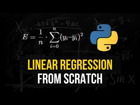
We'll build a linear regression model from scratch, including the theory and math. Linear regression is the most popular machine learning algorithm, and implementing it in python will help you understand how it works.

First, we'll cover the theory and the equation to calculate the coefficients. Then we'll implement the equation in python. We'll end by calculating the r squared value to figure out how well our regression fits the data.

We'll be using data from the Olympics to implement our algorithm. We'll try to predict how many medals a country will earn based on how many athletes it enters into the Olympics.

Chapters

00:00 Intro
00:20 Theory and equation
14:25 Python implementation
20:02 r-squared calculation

---------------------------------
Join 1M+ Dataquest learners today!
Master data skills and change your life.

[ninobach]

I recommend this video for those who understand the general concept of linear regression, but want to know what happens 'under the hood'

[namrata_roy]

Amazing tutorial. Difficult concepts were explained with such ease. Kudos team Dataquest!

[Mara]

This is absolutely amazing and great video. I can’t wait to see more great work

[sulaimansalisu]

Very explicit. You are a wonderful teacher. Thanks so much

[dataprofessor_]

this is a great tutorial. Beautifully explained.

[zheshipeng]

Thanks so much. Better than any E-books 🙂

[HIEUHUYNHUC]

Today you will my teacher. I'm from VietNam. Thank you so much <3. I'm looking forward to watching series logistics regression machine learning from you soon

[fassstar]

One correction, not relevant to the actuall regression, but should be said nonetheless. The number of medals one athlete can win is not limitted to one, rather it is limited to the number of events the athlete competes in (maximum of one per event). In fact, numerous athletes have one multiple medals in one Olympics. Just wanted to clarify that. Of course, from a certain number of athelets, it will be impossible for a smaller team to compete in as many events as the large team, making it more likely that the larger team wins more medals.

[im]

This guy is old, young, sleepy and awake all at the same time.

[ycombine]

"if you only enter one athlete, the most medals you can win is one" - Michael Phelps has entered the chat.

[anfedoro]

Great and very clear explanation. The only point missed in the end is the regression visualisation 😉. Nice to have both initial data and the regression plotted

[cclementson]

Is there a reason you chose to implement the normal equation over gradient descent? I'm quite curious as I am more familiar with gradient descent.

[iamgarriTech]

Why do we need to add those "1" when solving the matrix

[jeanb]

Hey, That is a great beatiful demonstration of linear regression. Thank you. But I didn't understand where prev_medals coming in building X matrix at the beginning?
some one can give to me explanation on apparution of these value inside the X matrix?

[bomidilakshmimadhavan]

Can you please make a video demonstrating the multivariate regression analysis with the following information taken into consideration?

Performs multiple linear regression trend analysis of an arbitrary time series. OPTIONAL: error analysis for regression coefficients (uses standard multivariate noise model).

Form of general regression trend model used in this procedure (t = time index = 0, 1, 2, 3, ..., N-1):

T(t)=ALPHA(t) + BETA(t)*t + GAMMA(t)*QBO(t) + DELTA(t)*SOLAR(t) + EPS1(t)*EXTRA1(t) + EPS2(t)*EXTRA2(t) + RESIDUAL_FIT(t),

where ALPHA represents the 12-month seasonal fit, BETA is the 12-month seasonal trend coefficient, RESIDUAL_FIT(t) represents the error time series, and GAMMA, DELTA, EPS1, and EPS2 are 12-month coefficients corresponding to the ozone driving quantities QBO (quasi-biennial oscillation), SOLAR (solar-UV proxy), and proxies EXTRA1 and EXTRA2 (for example, these latter two might be ENSO, vorticity, geopotential heights, or temperature), respectively.

The general model above assumes simple linear relationships between T(t) and surrogates which is hopefully valid as a first approximation. Note that for total ozone trends based on chemical species such as involving Chlorine, the trend term BETA(t)*t could be replaced (ignored by setting m2=0 in the procedure call), with EPS1(t)*EXTRA1(t) where EXTRA1(t) is the chemical proxy time series.

This procedure assumes the following form for the coefficients ALPHA, BETA, GAMMA, ...) in effort to approximate realistic seasonal dependence of sensitivity between T(t) and surrogate.

The expansion shown below is for ALPHA(t) - similar expansions for BETA(t), GAMMA(t), DELTA(t), EPS1(t), and EPS2(t):

ALPHA(t) = A0 <== Constant
<== 12-month
<== 6-month
<== 4-month
+ . . .
+ . . .
+ . . .

where A0, A1, A2, ... are constants, and t (t=1, 2, ..., n) is the time index (NO UNITS).

Trend models often use a particular harmonic expansion to represent the seasonalility of the action between T(t) and a particular surrogate. Shown below are two EXAMPLES of such chosen harmonic expansions for total ozone trend analyses [T(t) is a total ozone time series]:

1) Stolarski, Bloomfield, McPeters [1991] model:

ALPHA(t): A0, A1, A2, A3, A4, A5, A6, A7, A8 (const+12, 6, 4, 3mo)
BETA(t) : A0, A1, A2, A3, A4 (const+12mo+6mo)
GAMMA(t): A0, A1, A2 (const+12mo)
DELTA(t): A0, A1, A2 ( " " )
(no proxies other than QBO and SOLAR)

2) Randel and Cobb [1994] zonally asymmetric model:

ALPHA(t): A0, A1, A2, A3, A4, A5, A6 (const+12, 6, 4mo)
BETA(t) : A0, A1, A2, A3, A4, A5, A6 ( " )
GAMMA(t): A0, A1, A2, A3, A4, A5, A6 ( " )
DELTA(t): A0, A1, A2, A3, A4, A5, A6 ( " )
EPS1(t): A0, A1, A2, A3, A4, A5, A6 ( " )
(no proxies other than QBO, SOLAR, and an "EXTRA" proxy ENSO)

[guilhermesaraiva]

thanks for the lesson, but just a question, during the model the separation of x, y_train and x, y_test was not made, why would it not be necessary, and if it is necessary to do it, how would it be done?

thanks

[AndresIniestaLujain]

Would the solution for B be considered a least squares solution? Also, If we wanted to construct say a 95% confidence interval for each coefficient, would we take B for intercept, athletes, and prev_medals (-1.96, 0.07, 0.73) and multiply them by their respective standard errors and t-scores? Would the formula would be as follows: B(k) * t(n-k-1, alpha = 0.05/2) * SE(B(k)), or does this require more linear algebra? Great tutorial btw, thanks for the help.

[television]

Hi Vikas, which is better for GLM models in python: sklearn or statmodels package?

[joshwallenberg]

Do you have an example like this with multiple x-values or features?

[yousif_alyousifi]

Thank you for this video. Could you please share the ppt slides of this lesson?