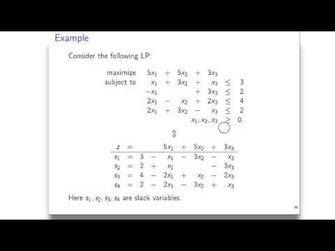
Linear Programming 18: The simplex method - Unboundedness

Linear Programming 18: The simplex method - Unboundedness

Abstract: We show how the simplex method behaves when the feasible region and the optimization function are unbounded.

This video accompanies the class "Linear Programming and Network Flows" at Colorado State University

We are following the book "Understanding and Using Linear Programming" by Jiří Matoušek and Bernd Gärtner

Our course notes are available at

[alexanderpoppe]

I just want to start off by saying this is an amazing series. It really helped me understand the intuition behind the simplex method. At the end of this video (8:15), there is a question about how we know which direction we followed when pivotting. My understanding is that every line drawn in the figure is the line where one variable is zero. So there are 4 lines (x1=0, x2=0, x3=0 and x4=0). These lines are not so difficult to draw when you use x1 as horizontal line and x2 as the vertical line. By setting x3 and x4 to zero in the equations from the equational form, you can draw this. Just watch out because the axis x1 is in fact the line where x2=0, which can be a bit confusing.

In the first step, we pivotted around x1 and kept x2 equal to zero. This means we are going along the horizontal line which represents x2=0. We keep on moving along this line which increases x1 until a boundary is reached. This boundary was here the line x3=0. So now the variables x2 and x3 are equal to zero.

In the next step we decided to increase x2 but keep x3 equal to zero. The only way to do that is by going along the line x3=0. Going straight up would mean we increase x2 and x3 and is not what we wanted so we go diagonally.

I hope this helps for anyone with the same question.