Creating Overall Progress Bar in Google Sheets

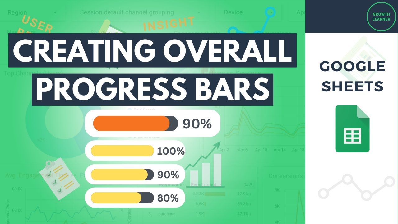
To create an overall progress bar in Google Sheets, we can use the sum function divided by the count function, along with the sparkline function. This allows us to visualize the progress data in a single bar, making it easier to track the overall progress.

Use the SUM function to calculate the sum of all the progress values in the specified range. The SUM function adds all the numbers in a range of cells.

Here's an example of how you can use the SUM function to calculate the sum of the progress values in a range:

=SUM(A1:A10)

In this example, the range A1:A10 contains the progress values. The SUM function will return the sum of all the numbers in this range.

To count the total number of progress values in the specified range in Google Sheets, you can use the COUNT function. The COUNT function counts the number of cells in a range that contain numbers or dates.

Here's an example of how you can use the COUNT function to count the progress values in a range:

=COUNT(A1:A10)

In this example, the range A1:A10 contains the progress values. The COUNT function will return the total count of cells in this range that contain numbers.

To create an overall progress bar from multiple progress values, you can divide the sum of the progress values by the count of progress values.

Here's an example of how you can calculate the overall progress using the sum and count functions:

=SUM(A1:A10)/COUNT(A1:A10)

In this example, the range A1:A10 contains the progress values. The SUM function calculates the sum of all the progress values, and the COUNT function calculates the total count of progress values. The result of the division gives you the overall progress.

Lastly, if you want to visualize the overall progress using a sparkline, you can use the SPARKLINE function. The SPARKLINE function creates a miniature chart to represent data in a single cell.

Here's an example of how you can use the SPARKLINE function to create a sparkline for the overall progress:

=SPARKLINE([overall progress data],{"charttype","bar";"max",100%;"color1","[color]";"empty","zero"})

The SPARKLINE function takes the result of the division (overall progress data) as its argument. It will create a sparkline chart in a single cell to represent the overall progress visually.

Disclosure: Some of the links are ‘affiliate links.' This means if you click on the link and purchase a product, I'll receive a commission at no additional cost to you.

[patricejauffret]

Hello, for the european's people there is an other syntax, like this - Thx you for your video !

[AfrhilDelgado]

Thank you for posting the code in the description! I tried to apply the code from your old video but didn't work because I missed the comma after the overall progress data. Now it works. This is a big help! Thank you!

[useyourdelusionand]

Thanks for the knowledge Mitch Hedberg.

[jmjelfe]

Is there a way I can create a Sparkline for individual statuses from a dropdown list? This way the progress bar will update based on the status picked from the drop down menu.

[edengills]

Is there a way to tie the check box to automatically be taken as 100% once checked off without the need for making a column of percentages for non-sum items? For example, if I am crossing to-do items off a list and want to see my progress?

[TypeWriterDLC]

Is there a way to display the percentage text in the same cell as the progress bar?

[definetheterms]

Is there a way to have the progress bar completely fill up the cell? Instead of having the white border around the bar?

[baxter]

Hi. How can i show that by completed a task will only contribute a certain percentage in overal progress bar? Every task will have their weightage.

[Toasted_Sandwiches]

Is there a way to extend the progress bar into other cells so i can have like 3 cells be 1 progress bar?

[marjim]

Hi great video thanks for sharing. Is there not a way to add a secondary color to the progress bar like you would for a normal progress bar, for example like this: =SPARKLINE({'Point Tracking'!D27, 'Point Tracking'!E27}, {"charttype", "bar";"color1", "#6aa84f";"color2", "#f6b26b"})

I'm finding it difficult to add color 2 to the formula, thanks in advance

[elbruzx]

Thank you sir. I have question, how if I want to make gradient color when value lower than 50%, it will color green, and if value higher than 50% it will red.

[claireantonette]

Hi, is it possible to make 1 progress bar with 3 variables in it? I want to make a tracker for my lessons based on the drop down list: Recalled, Familiar, Mastered.

[OnlyNeedJuan]

I want the entered value to dynamically change the color of the chart, say I have 1/255, that would be red, but 255/255 that would be bright green, is that possible?

[oufcoxm]

Hi, is there any way to make the progress bar go forward based on how many dropdowns have one specific option? For example, 100% = all dropdowns in the column have "Passed". Thanks!

[fldzady]

sir, can you help me. Idk what's wrong with my laptop but when i tried to make this sparkline i can't use any comma, instead i can only use semicolon. Can you give me example for this case?? with semicolon as comma?
Thankyou so much

[AronM]

Is there a way to have multiply colours (in traffic light settings)

[MyatThinzarMonica]

How to show the text in this sparkline ? thank you

[yhliqbe]

This does not seem to work ... I get error for only giving 1 "data" cell - where I have my overall status - and, I get some weird line chart representation versus a progress bar as seen on your screen...

[Zairin.]

would be nice if you told us how to enter a hex value instead of a color also my formula is saying its expecting another data point.

[davidellis]

The video image has rounded edges on the progress bars. Is there a way to do that in google sheets?