R Tutorial: Data Visualization in R (part 3)

Most base R graphics functions support many optional arguments and parameters that allow us to customize our plots to get exactly what we want. In this chapter, we will learn how to modify point shapes and sizes, line types and widths, add points and lines to plots, add explanatory text and generate multiple plot arrays.

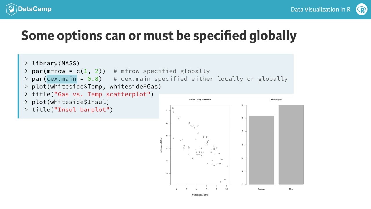
All base R graphics functions support a variety of optional parameters that allow us to change key plot details. These graphics parameters can either be set locally, as part of the call to a specific plotting function, globally through a call to the par() function, or in some cases, through both of these methods.

Here is an example of a global parameter that can only be set by the par() function: mfrow sets up an array of multiple plots, and this must be done before any of these plots can be generated. In this case, we have specified par(mfrow = c(1, 2)) to set up an array of two side-by-side plots. Part of Chapter 4 is devoted to a discussion of the effective use of multiple plot arrays like this one.

Another example of a parameter that can be specified either way is pch, which defines the shapes of the points in either one plot (if the parameter is specified locally) or in all subsequent plots (if the parameter is set globally). Note that if we specify pch globally via the par() function, we are effectively changing the default value from pch = 1 (open circles) to something else of our choosing.

An example of a strictly local graphics parameter is the type argument in the plot() function, which specifies the kind of plot that will be drawn (e.g., points, lines, or points overlaid on lines). Here, we see the effect of specifying type = 'o' to obtain points overlaid on lines.

Another important aspect of base R graphics is the distinction between "high-level" graphics functions like plot() that generate an initial plot, and "low-level" graphics functions like points(), lines(), or text() that add details to an existing plot.

All of these functions support both local and global optional parameters that can be used to help us make plots look the way we want them to look.

In this example, the high-level function plot() is first called to create the initial plot, locally setting type, pch, xlim, ylim, xlab, and ylab to get the type of plot and point shapes we want, the x- and y-axis limits we want, and the x- and y-axis labels we want. Note that this initial plot has lines overlaid with solid circles, and by specifying xlim and ylim explicitly, it leaves room on the plot for the second line.

This second line is added by the low-level graphics function lines(), again as a line overlaid with points through the local type = 'o' specification, where the points are represented as open circles through the specifiction pch = 1.

One of the valid values for the type parameter is "n", which specifies "no plot." This option is useful in cases where we want to initially set up axis limits, labels, and other plot parameters using a high-level graphics function like plot() and then add points or lines using the low-level points() or lines() functions.

Now it's your turn: the following exercises ask you to, first, explore the range of graphics parameters that can be set using the par() function, and then create plots using both low-level and high-level graphics functions.