R Tutorial: Descriptive Statistics

---
Descriptive statistics are useful prior to modeling any data, and longitudinal data are no exception. This lesson will explore a few descriptive analyses that help understand longitudinal data better before modeling it.

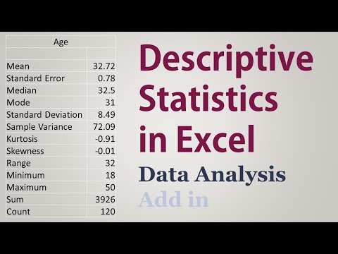
Numeric summaries of the data are a great way to explore longitudinal data and include calculating the mean, median, minimum, maximum, and standard deviation of the variable of interest. It is useful to do this overall across all time points, but often these descriptive statistics are most useful when broken down by time or other predictors that are of interest.

The dplyr package, from the tidyverse, has great tools for exploring numeric summaries. The summarize and group underscore by functions will be used most frequently.

Here we use the BodyWeight data and group the analysis by the time variable. Then the summarize function computes the mean, median, minimum, maximum, and standard deviation of the outcome variable. Note, the na dot rm argument is specified for each function to remove any missing data prior to calculating the descriptive statistic. If this is not specified and there are missing data, NA will be returned. The number of missing observations and total observations at each time point are also returned. This information demonstrates the balanced or unbalanced nature of the data and the amount of missing data compared to the total number of observations.

The numeric summary output has a single row for each time, with the time shown in the first column. The general trajectory can be determined from the mean and median values. In this case, there is evidence that the rats tend to increase in weight over time. Additionally, the median tends to be smaller than the mean, suggesting there may be a rat or two with extreme weight values pulling the mean above the median. The minimum and maximum can help identify unusual or extreme values. Without further context, these values do not seem unusual. The standard deviations have some variation at each time point, but should be relatively similar across time to meet model assumptions, as is the case here. Finally, there are no missing data.

Exploring the distribution of the outcome variable at each time point can also provide valuable insight. Violin plots and sina plots are useful figures for this. We will use violin plots, as these are in the ggplot2 package natively.

The following code generates violin plots for each unique time point and diet. Note the use of the factor function with the time variable, otherwise, all the time points would be pooled into a single violin plot, which would ignore the time trend. The xlab and ylab functions are used to specify the x-axis and y-axis labels and the theme underscore bw function determines the theme.

The resulting figure shows skewed distributions for rats in diets one and three, but these two diets have similar variation. Diet two differs from the others with larger variation at each time point.

Time to practice your understanding of descriptive statistics.

#DataCamp #RTutorial #Longitudinal #Analysis #Descriptive #Statistics