Transfer Function to State Space

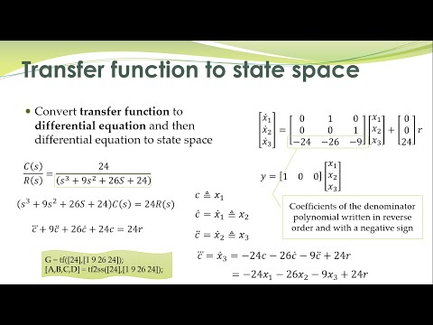
In this video we show how to transform a transfer function to an equivalent state space representation. We will derive various transformations such as controllable canonical form, modal canonical form, and controller canonical form. We will apply this to an example and show how to use Matlab’s tf2ss function to help with this transformation. Finally, we use Simulink to show that all representations yield the same input/output relationship.

Topics and timestamps:
0:00 – Introduction
1:17 – Controllable canonical form
27:16 – Modal canonical form
41:11 – Other canonical forms via similarity transformations
51:07 – Controller canonical form via tf2ss
55:41 - Conclusions

#Matlab #Simulink

#Control #ControlTheory

[husnimuttaqin]

bro was so helping me to finish my collage. thank you for detail explanation

[seanstocker]

AE 511: This was a great video. In past classes I had a hard time understanding the relationship between state-space, transfer functions and ODE's and how they are related to the physical system they represent. After watching this and the previous video on moving from state-space to transfer function it finally clicked and makes sense.

[nathanlipshutz]

AE511: It never occurred to me that you could have infinite, or even multiple, state space representations for a given system. Interesting characteristic!

[Qaidi_]

Thanks for such an amazing Video. Please also make video on Model Predictive Control Implementation on a Real Plant

[melissawells]

The reminder on matrix multiplication properties was useful to follow through on the derivation of G tilde

[Jnglfvr]

At 54:32 the ONLY difference between "controllable" canonical form and "controller" canonical form is the ordering of the states. So, e.g. in controllable canonical form (say for a third order system) we take x1 = y; x2 = y', x3 = y''. Whereas in controller canonical form we take x1 = y'', x2 = y' and x3 = y. The states are simply labeled in reverse order but otherwise are IDENTICAL. They are surely linked by a similarity transformation (as they must be) but that transformation does not take linear combinations of the states and rearranges them but rather simply reverses their ordering. In the case of a 2X2 matrix as in your example they are related by the matrix V = [0 1;1 0].

[ahungryflyer]

AE511: Is the infinite amount of state space representations for a specific system due to the fact that the state vectors themselves can differ across state space representations? Great video that is helping to clear up the state space - laplace domain relationship.

[devmakwana]

What about complex conjugate roots and multiple similar real poles i.e (s+1)^2. Thank you

[sebasA]

Hi, in the min 15:49 what if n=4 and m=2? how can I represent the vector x(t) on the output equation? Is fine if I put a d^3(y)/d(t)=0? Thanks

[sethwhittington]

AE511: At time stamp 32:42 I'm not sure how you went from the block diagram to writing differential equations...?

[lucasharlen]

33:36, if the denominators of the transfer function were repeated
Ex (s+1)(s+3)(s+3)

The resultant partial fraction would be A/(s+1) + B/(s+3) + C/(s+3)²

I would end up with a 2nd order differential equation for the 3rd equation
How would I draw up the space state equation from this?

[nhutnguyen]

Hello sir, i still wonder what we can do if numerator and denominator have the same level of s, example: s^4/s^4 Thanks you