OFFSET function in Excel

Why would you use the OFFSET function in Excel, and how do you use the OFFSET function in Excel?

A very common reason why people use the OFFSET function in Excel, is having standardized reporting with changing datasets. For example, the two charts that you see in this Excel workbook represent the number of monthly views on my Finance Storyteller YouTube channel on the left, and the number of quarterly views on the right. Using the dropdown box at the top, I can switch between the years: 2017, 2018, 2019, 2020, and future years once that data is available. The views data and month labels for the blue line on the left always get pulled from cells K21 through L32, whatever year I select. The views data and quarter labels for the blue bars on the right always get pulled from cells M21 through N24, whatever year I select. You could do the same with your charts on revenue, expenses, margins, headcount, or whatever the metric is that you are tracking. The reporting is standardized and stays in the same format. I just want to add new rows and new columns to the dataset when data becomes available for new time periods. On a monthly basis, I just add the latest results, without having to update any formulas. That’s what the OFFSET function in Excel is doing for us: OFFSET is used here as the linking pin between dataset and charts.

⏱️TIMESTAMPS⏱️
0:00 OFFSET function in Excel
1:39 How the OFFSET function works
3:02 OFFSET function arguments
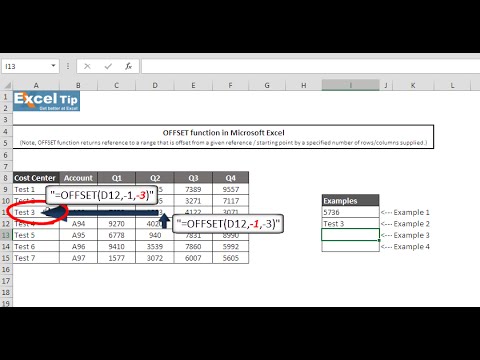
5:19 OFFSET with negative values
5:57 OFFSET error messages REF and VALUE
6:36 OFFSET function nested in SUM
8:01 COUNTA function nested in OFFSET
9:12 Dynamic chart titles

Let’s hide the charts for a moment, and show you how the #OFFSET function works. If we change the year in cell F1, then the data in columns L and N is changing. The original dataset, which is in cells A20 through I32, does not change. The OFFSET function doesn't actually move any cells; it just returns a reference. The central cell that makes things happen is L20, which is a calculation of the offset in number of years versus the first year in the table. If we go to Formulas – Trace Dependents, we see that L20 impacts each of the months in cells L21 through L32, and each of the quarters in cells N21 through N24.
If the year is 2016, then the offset is zero, and the data in column L is the same as in column B.
If the year is 2017, then the offset is one, and the data in column L is the same as in column C.

Let’s get into the detail of the function arguments of the OFFSET function. Let’s review those with the year set to 2017. Select cell L21, go to the Home tab – Functions – More Functions, and review the function arguments in the dialog box. You use OFFSET to find certain data for you, so you need to tell the function where to go for that data. The first argument is called Reference. This is like defining a “base station” for the expedition, the starting point. I took the top left cell of the table: B21. I could also have taken a range of cells, like B21:I21. This would have given me the same result, as #Excel would take the left-most cell out of that range as the starting point. Next argument is Rows. How many rows, up or down, would you like to go from starting point B21? Rows can be positive (which means below the starting reference) or negative (which means above the starting reference). In this OFFSET function, zero, we want to stay on the same row, which is row 21. Next is Columns. How many columns, left or right, would you like to go from starting point B21? Columns can be positive (which means to the right of the starting reference) or negative (which means to the left of the starting reference). Here I didn’t input a fixed number of columns, I made this dynamic by referring to cell L20, which in turn depends on the year selected from the dropdown box. I have locked column L and row 20 in this function argument with $ signs, as we don’t want this column and row reference to change when we copy the cell. Then there are two optional arguments: height and width. How high, in number of rows, would you like the returned reference to be. How wide, in number of columns, would you like the returned reference to be. We go with 1 and 1, the size of a single cell. This formula I have then copied down the column for each of the months.

Philip de Vroe (The Finance Storyteller) aims to make accounting, finance and investing enjoyable and easier to understand. Learn the business and accounting vocabulary to join the conversation with your CEO at your company. Understand how financial statements work in order to make better investing decisions. Philip delivers #financetraining in various formats: YouTube videos, livestreams, classroom sessions, and webinars. Connect with me through Linked In!

[nabeelal-shammari]

You are sir an absolute legend, keep up the good work.

[seuchyea]

Hello, can you help me with my business studies case study? I don’t really know how to do it (the topic is costs, scale of production and break even analysis)

[jamiuadeniran]

Please how did you create this, was it through validation?

[dennismoe]

You sound a lot like the Eastory history channel.