Conditional Formatting Google Sheets Tutorial 🎨

Learn the basics of Conditional Formatting in Google Sheets. Format based on a single condition, create color scales and start using custom formula.

0:55 - Google Sheets basic formatting
2:55 - Conditional formatting in Google Sheets
4:33 - Combine conditional formatting with data validation
6:37 - Color scale in Google Sheets
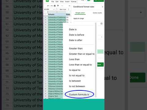
9:06 - Conditional formatting using the custom formula: highlight row
11:35 - Apply conditional formatting to multiple worksheets
12:06 - Railsware color-coding approach

✅ Subscribe to Railsware and learn the most efficient product management tools with us!

[iusmanasif]

Just become a regular watcher and a subscriber :)

[aubreycampbell]

This was incredibly helpful-- thank you.

[josetomevalbuena]

Hello. I have seen your first video and learned many things that I did not know about Google Sheets. Now I'm looking at "Conditional Formatting", where you use the "Add-ons" tab that I don't have in my spreadsheet, and that has been replaced by the "Extensions" tab. My question is if the latter tab is similar to the first, and if not, what should I do? Thanks.

[debbiehines]

I would like to know if you can format condition the workbook tab, once the data in the sheet is fill in?

[GBpetkov]

I am trying to figure out if I can do a conditional formating that will automatically change based on the value of another cell which also changes automatically. This is the cell that I want to link my conditional formating to =COUNTIF(A4:A1002, "<>") I have few other columns with =countif(C4:C1002, true). In column A I am adding data manually, that will change the value in the cell with the first formula for example to "100" I want to make the background of the cells with the second formula change colors from red to green when the number is closer or equal to the value in the cell with the first formula.
In every column with the second formula, there is a specific number of tasks which need to be done, that number is always changing and it is shown in the cell with the first formula

[rodrigocezar]

How can I do the same as you did? but in addition another condition, an "AND" if both were true, the condition is done.

[andreaguerri]

Hi Anastasia, I have a problem with a conditional formatting formula. I tried to type a formula with reference to a different sheet, for example: = database!A2, but it generates an error, did I miss something? Sorry for my english, I'm italian :o)

[sanjaybarge]

I WANT TO PROTECT COMPLETE SHEET BUT EXCEL 1000 CELLS LOCATED DIFFERENTLY PLEASE GUIDE

[THE_CHOAS_ENGINE]

I think I found a bug or something. I have a cell called "CLOSING %"... and it is capable of showing a number between 0% and 100% based on a derived calculation from other cells. It's actually in decimals from 0.00 to 1.00 and I just format it as a %... Either way... I want as RULE 1 = 0% to be red... and up to 20% yellow. So a smooth transition from Red to Yellow over 20%. THEN... I want to add RULE 2 to go from Yellow at 21% up to 50% which is GREEN... so that any closing % over 50% is just green and anything from 20% to 50% is a smooth transition from yellow to green.... in affect and from 0% to 50% it runs through 2 smooth transitions of colors instead of just 1 rule in which I believe the color transitions jump more and not so smooth.

But its not working it only really follows the first rule and anything over 20% just stays yellow!?

[chinmaymathur]

can you please explain why the two cells of column A were highlighted instead of column H earlier?

[TheCekobi]

you sound like blackwidow of the avenger: end game