filmov
tv
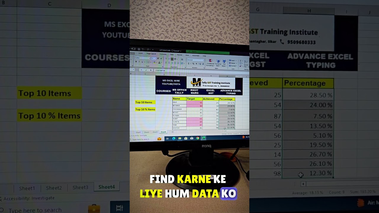
Conditional Formatting Top/Bottom Rules in excel | Top/Bottom 10 Items ,Top 10 % Rules #msexcelwire
Показать описание
IN This video step-by-step process of top/bottom rule to automatically highlight the highest values . This function use step by step with multiple Conditional Formatting: Highlighting Rules Top 10% Using Top/Bottom Rules so Conditional formatting is a powerful tool that allows Conditional Formatting, Top/Bottom Rules in excel, Top 10 Items ,Top 10 %, Bottom 10 Items ,Bottom 10 % ,Above Average, Below etc.
Learn about how to use The Conditional Formatting TOP/Bottom Rules in Excel allows the user to highlight the cell that satisfies the criteria (Top 10 items..., Bottom 10 items..., Top 10%..., Bottom 10%..., Above Average... or Below Average...) in the selected range."
Excel Top/Bottom Rules?
Highlight top and bottom values with built-in rule
The fastest way to highlight top 3, 5, 10 (or bottom n) values in Excel is to use an inbuilt conditional formatting rule. Here's how:
1. Select the range in which you'd like to highlight numbers.
2. On the Home tab, in the Styles group, click Conditional Formatting.
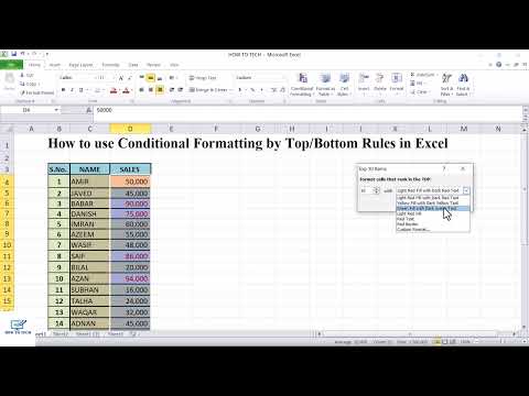
3. In the drop-down menu, pick Top/Bottom Rules, and then click either Top 10 Items… or Bottom 10 items…
Top/Bottom Rules is a part of Conditional Formatting that enables you to apply formatting to cells that satisfy a statistical condition in the range.(for example, below average, within top 10 items, or below 10%, etc.).
Top 10 Items
To highlight the cells with one of the colour options based on the cell value that satisfies the criteria of top values in the selected range.
Top 10%
To highlight the cells with one of the colour options based on the cell value that satisfies the criteria of top percent of values in the selected range.
Bottom 10 Items
To highlight the cells with one of the colour options based on the cell value that satisfies the criteria of bottom values in the selected range.
Bottom 10%
To highlight the cells with one of the colour option based on the cell value that satisfies the bottom percent of values in the selected range.
Above Average
To highlight the cells if the cell value is above the average value in the selected range.
Below Average
To highlight the cells if the cell value is below the average value in the selected range.
On the Home tab, in the Style group, click the arrow next to Conditional Formatting, and then click Top/Bottom Rules. Select the command you want, such as Top 10 items or Bottom 10 %. Enter the values you want to use, and then select a format.
conditional formatting in excel, Bottom 10 Items, how to make a new conditional formatting rule in excel, create new conditional formatting rule, advanced custom formatting, excel custom formatting conditional, conditional format, conditional formatting in excel, MS Excel - Conditional Formatting, conditional formatting in excel with example, Conditional Formatting, top/bottom in excel, top/bottom in ms excel, advanced conditional formatting in excel, formatting rules, conditional formatting, top/bottom in excel, conditional formatting formula, top bottom in excel, top bottom rules in excel in hindi, Top/Bottom Rules in excel, conditional formatting top bottom rules in excel, conditional formatting with different colors, ms excel advanced conditional formatting, conditional formatting in excel with color, conditional formatting in excel in hindi, top bottom rules in excel, Bottom 10 %, excel custom formatting, how to use top bottom rules in excel, custom formatting color, top/bottom in ms excel, color row in excel by conditional formatting, excel conditional formatting color, conditional formatting in excel, conditional formatting, excel conditional formatting, Top 10 Items, conditional formatting in excel based on another cell, conditional formatting excel,
Thanks For Watching
Sikar Msexcel Wire
Grow Your Skills With Excel Wire .
Learn 👉 Rkcl ।। Rscit ।। Basic Tally Gst
।। Marg Erp ।। Accounting।। Typing ।। Excel ।। Advance Excel ।। Google Sheet Etc
|| Microseft Sikar ||
Computer Training Institute
📞 : Call For Enquiry - 9509680333
.
.
📍: Location - Near Clock Tower ,Sikar
Learn about how to use The Conditional Formatting TOP/Bottom Rules in Excel allows the user to highlight the cell that satisfies the criteria (Top 10 items..., Bottom 10 items..., Top 10%..., Bottom 10%..., Above Average... or Below Average...) in the selected range."
Excel Top/Bottom Rules?
Highlight top and bottom values with built-in rule
The fastest way to highlight top 3, 5, 10 (or bottom n) values in Excel is to use an inbuilt conditional formatting rule. Here's how:
1. Select the range in which you'd like to highlight numbers.
2. On the Home tab, in the Styles group, click Conditional Formatting.
3. In the drop-down menu, pick Top/Bottom Rules, and then click either Top 10 Items… or Bottom 10 items…
Top/Bottom Rules is a part of Conditional Formatting that enables you to apply formatting to cells that satisfy a statistical condition in the range.(for example, below average, within top 10 items, or below 10%, etc.).
Top 10 Items
To highlight the cells with one of the colour options based on the cell value that satisfies the criteria of top values in the selected range.
Top 10%
To highlight the cells with one of the colour options based on the cell value that satisfies the criteria of top percent of values in the selected range.
Bottom 10 Items
To highlight the cells with one of the colour options based on the cell value that satisfies the criteria of bottom values in the selected range.
Bottom 10%
To highlight the cells with one of the colour option based on the cell value that satisfies the bottom percent of values in the selected range.
Above Average
To highlight the cells if the cell value is above the average value in the selected range.
Below Average
To highlight the cells if the cell value is below the average value in the selected range.
On the Home tab, in the Style group, click the arrow next to Conditional Formatting, and then click Top/Bottom Rules. Select the command you want, such as Top 10 items or Bottom 10 %. Enter the values you want to use, and then select a format.
conditional formatting in excel, Bottom 10 Items, how to make a new conditional formatting rule in excel, create new conditional formatting rule, advanced custom formatting, excel custom formatting conditional, conditional format, conditional formatting in excel, MS Excel - Conditional Formatting, conditional formatting in excel with example, Conditional Formatting, top/bottom in excel, top/bottom in ms excel, advanced conditional formatting in excel, formatting rules, conditional formatting, top/bottom in excel, conditional formatting formula, top bottom in excel, top bottom rules in excel in hindi, Top/Bottom Rules in excel, conditional formatting top bottom rules in excel, conditional formatting with different colors, ms excel advanced conditional formatting, conditional formatting in excel with color, conditional formatting in excel in hindi, top bottom rules in excel, Bottom 10 %, excel custom formatting, how to use top bottom rules in excel, custom formatting color, top/bottom in ms excel, color row in excel by conditional formatting, excel conditional formatting color, conditional formatting in excel, conditional formatting, excel conditional formatting, Top 10 Items, conditional formatting in excel based on another cell, conditional formatting excel,
Thanks For Watching
Sikar Msexcel Wire
Grow Your Skills With Excel Wire .
Learn 👉 Rkcl ।। Rscit ।। Basic Tally Gst
।। Marg Erp ।। Accounting।। Typing ।। Excel ।। Advance Excel ।। Google Sheet Etc
|| Microseft Sikar ||
Computer Training Institute
📞 : Call For Enquiry - 9509680333
.
.
📍: Location - Near Clock Tower ,Sikar
 0:03:26
How to Use Top / Bottom Rules Conditional Formatting in Excel - Tutorial
 0:05:54
6.8 Conditional Formatting (Top Bottom Rules) in Excel | Excel tutorial for Beginner 2022
 0:04:36
How to use Conditional Formatting Top Bottom Rules from A to Z
 0:03:55
Conditional Formatting in excel 10 Items , Top 10 % Rules | Top/Bottom Rules in excel @msexcelwire
 0:04:30
Conditional Formatting Top Bottom Rules Excel | Conditional Formatting in Excel
 0:05:57
The Power of Top/Bottom Rules | Excel Conditional Formatting | Highlighting Top and Bottom Values
 0:00:35
Conditional Formatting Top Bottom Rules Top 10 Values
 0:05:28
Mastering Excel Conditional Formatting: Highlighting Top 10% Using Top/Bottom Rules
 0:08:16
'Master Conditional Formatting in Excel | Beginner to Advanced Guide'
 0:01:15
How to use Conditional Formatting by Top/Bottom Rules in Excel
 0:00:46
Conditional Formatting Top/Bottom Rules in excel | Top/Bottom 10 Items ,Top 10 % Rules #msexcelwire
 0:02:27
022. How to highlight top or bottom 10 values using conditional formatting! in 2 min! | EXCEL
 0:00:47
Conditional Formatting:Top/Bottom Rules:How to highlight bottom 10 percent items in excel?#shorts
 0:07:22
Conditional Formatting-MS Excel|Top Bottom Rules in excel|Excel Basic for beginners in Hindi |PART 3
 0:06:43
Conditional Formatting in Excel Tutorial
 0:00:54
Conditional Formatting top/bottom rules & highlight cells #Conditionalformatting #MSExcel2019
 0:02:42
Excel Home Styles Conditional Formatting Top Bottom Rules
 0:00:16
CONDITIONAL FORMATTING(Top/Bottom Rules) - MS Excel 2021 #shorts
 0:04:27
Conditional Formatting: Highlight Top Bottom Rules
 0:05:20
how to use conditional formatting in excel | Top bottom rules in excel | Conditional formatting
 0:05:16
Excel Conditional Formatting Top Bottom Rules
 0:06:57
Conditional formatting Top Bottom Rules
 0:02:56
Conditional Formatting Top Bottom Rules for numbers
 0:00:29
Conditional Formatting in Excel | Highlight Marks Pass/Fail #shorts #excel
Комментарии