Intro Stat, Lec 14B, Normal Approx to Binomial, Poisson RVs, Confidence Intervals for Pop Mean

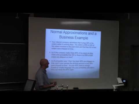
(0:00) Review Normal approximation to a Binomial distribution problem from the end of Lecture 14A.
(3:32) Word of warning about whether a binomial distribution is the best model for the on-time shipping example.
(4:30) Poisson random variables (highlight the similarities and differences with binomial RVs).
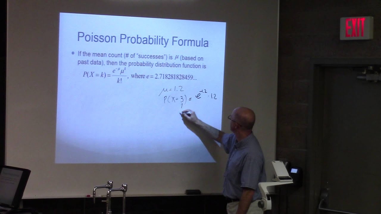
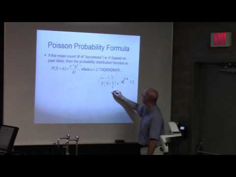
(5:46) Poisson probability formula.
(6:00) Example: compute P(X = 3) when mu = mean = 1.2.
(8:25) Using =POISSON(k,mean,cumulative) on a spreadsheet.
(9:15) Compute the probability distribution on a spreadsheet.
(11:43) Compute the mean as a summation on the spreadsheet and confirm it equals the stated value of the mean mu.
(12:29) Special formulas for the mean and standard deviation that only work for Poisson RVs.
(14:00) Other slides with graphs to look at and think about. Approximate probabilities on two graphs for a Poisson distribution with mu = 1.2.
(15:21) Confidence intervals to estimate a population mean when we assume (unrealistically) that the population standard deviation is known. We are starting Chapter 6. The most important chapter: it contains the fundamentals of inferential statistics.
(19:23) The logic of confidence intervals (using the Central Limit Theorem).
(22:38) A bit of algebra to restate the probability for a 95% confidence interval.
(24:45) For more accuracy, we will use 1.96 instead of 2 as the 95% confidence interval multiplier in this chapter. Show the formula for the confidence interval in both "plus or minus" notation and in (open) "interval notation".
(25:50) Numerical example to illustrate the connection between the different notations.
(27:25) Encouragement to write answers with both notations to increase understanding. Ultimately, the calculations are not too hard, but the concept is challenging to understand.

#normalapproximation #poissondistribution #confidenceinterval

AMAZON ASSOCIATE
As an Amazon Associate I earn from qualifying purchases.