filmov
tv
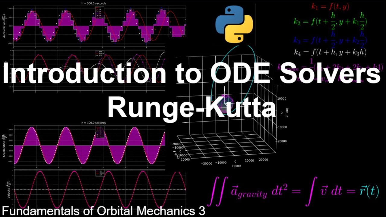
Introduction to ODE Solvers (Runge-Kutta) | Fundamentals of Orbital Mechanics 3
Показать описание
In this video we’ll be going over how ordinary differential equation (ODE) solvers work including Euler’s method and the famous Runge-Kutta methods. Higher order Runge-Kutta methods use multiple evaluations of the derivative function in order to estimate the solution to said differential equation, which can also be thought of as the area under the curve of the derivative function.
We’ll also be discussing how time step affects error and why it makes sense to use adaptive step sizing methods based on how quickly the derivative is changing throughout the propagation.
We start with the simplest method of numerically solving a differential equation (called Euler’s method, or Runge-Kutta 1st order method). To solve, you evaluate the derivative of a function at some time, and you assume that the derivative is constant for the whole timestep and propagate forward with that constant derivative. We immediately see that our estimate of the solution is quickly building error, since the slope is continuously changing, but we are assuming the slope to be constant within time steps.
We can also think about this method as estimating the area under the curve of the derivative function, where the area under the curve estimate would be equal to the area of a rectangle who’s height is the derivative function at that time and its width is the time step. So here, the next estimate of the velocity is equal to the previous estimate plus the area under the curve of the acceleration function, which is also equal to the cumulative area under the curve of acceleration.
Instead of just evaluating the derivative once like in euler’s method, higher order Runge-Kutta methods evaluate the derivative multiple times in order to get a better estimate of how much the function changes over one time step. Runge-Kutta are a family of methods because you can choose any order you want, with the most common being 4th and 5th order.
The derivative evaluations are summed up to a weighted mean, then we use that weighted mean estimate of the derivative between now and the next time step to update our estimate of the function at the next time step. So to summarize, Runge-Kutta methods use weighted averages of derivative evaluations throughout the given timestep.
Even though higher order runge-kutta methods take better estimates of derivatives, they still will grow error over time. ODE solvers therefore make trades between function evaluations (which translate to compute time) and error from the true solution of the differential equation (which is accuracy of the solution).
But, instead of just using the same step size the whole time, you can change that step size based on the dynamics of the system.
When the solution to a differential equation is approximately linear, this means that the derivative is roughly constant, so even just using Euler’s method will yield you a good estimate of the solution with large time steps. Therefore, when the derivative is relatively constant, an ODE solver can use larger time steps without sacrificing accuracy.
On the other hand, when the derivative is changing rapidly, the solver should use smaller time steps in order to maintain accuracy. This adaptive step sizing is why you’ll sometimes see when a solver errors, the message will say “step size becomes to small”, because even with a step size near machine epsilon (floating point limits), the solver can’t achieve its tolerance constraints.
Links to the Space Engineering Podcast (YouTube, Spotify, Google Podcasts, SimpleCast):
Link to Orbital Mechanics with Python video series:
Link to Spacecraft Attitude Control with Python video series:
Link a Mecánica Orbital con Python (videos en Español):
Link to Numerical Methods with Python video series:
#odesolver #runge-kutta #orbitalmechanics
 0:08:59
Introduction to ODE Solvers (Runge-Kutta) | Fundamentals of Orbital Mechanics 3
 0:02:40
Learning the Runge-Kutta Method 1. Basic Runge-Kutta
 0:02:54
Ordinary Differential Equations: Intro to ODE Solvers
 0:17:11
Introduction to ODE solvers
 0:14:46
2WN50 Module 7: ODEs (IVPs) - Runge-Kutta methods
 0:09:35
ODE Solvers (Runge-Kutta, Adams) in Orbital Mechanics / Astrodynamics | SEP Clips 8
 0:05:15
RUNGE-KUTTA: SHORT Explanation + Python script
 0:06:32
Using Runge Kutta ode45 to solve a simple first order differential equation in Matlab
 0:09:17
7.2.1-ODEs: Adaptive Runge-Kutta
 0:02:54
A C++ Program for Solving ODEs Using the Classical Runge-Kutta Method
 7:53:35
Introduction to Ordinary Differential Equations (Free Full Course)
 0:12:47
Dense or Continuous Output for ODE Solvers
 0:01:26
Introduction Nonlinear optimal control with Excel Solver Runge-Kutta
 0:09:01
Supplement: Using ODE45 & Runge-Kutta methods
 0:30:10
Programming for AI (AI504, Fall 2020), Practice 14: Neural Ordinary Differential Equations
 0:02:28
Solving ODE problem using Runge-Kutta Method and simulink
 0:13:34
The Ways ODE Solvers Fail
 0:18:26
Runge-Kutta for Coupled Ordinary Differential Equations -- C++ Implementation
 0:20:50
Euler's Method Differential Equations, Examples, Numerical Methods, Calculus
 0:06:40
Runge-Kutta solution to a System of ODEs
 0:10:07
Euler's method | Differential equations| AP Calculus BC | Khan Academy
 0:01:04
Ordinary Differential Equations: Production ODE Solvers Quiz Solution
 0:12:12
Runge Kutta 4th order method for ODE2
 0:07:16
CBE 330 09 09 - Comparing Matlab ODE solvers
Комментарии