Calendar Template In Excel - PART 1 - Excel Tips and Tricks

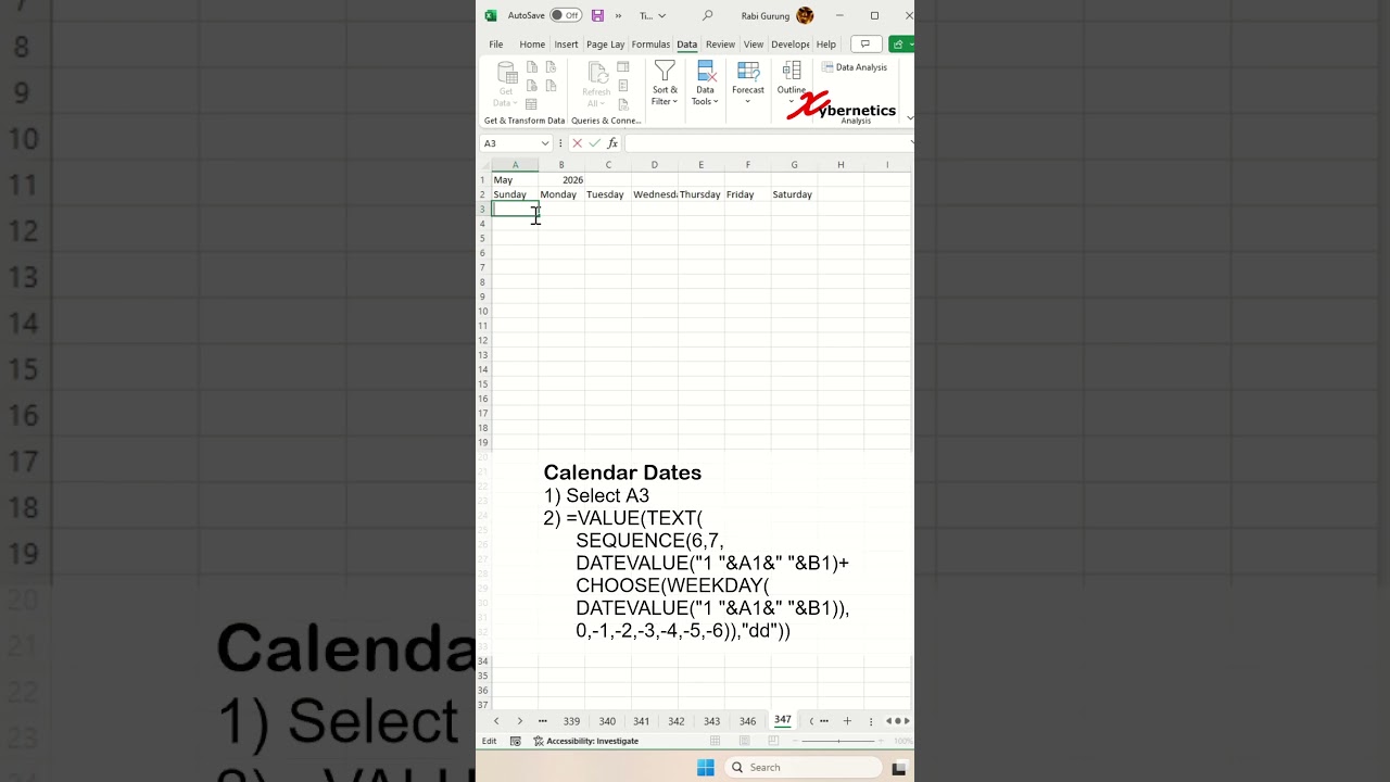
Create calendar template in Excel.

Excel provides a convenient calendar template that users can easily access to organize their schedules efficiently. By selecting the "File" tab, then choosing "New," individuals can explore a variety of templates, including pre-designed calendars. Furthermore, Excel offers a built-in scheduling template that streamlines the process of planning and managing tasks. Users seeking a calendar view can transform their Excel spreadsheet by utilizing the program's conditional formatting and data validation features, allowing them to customize the appearance according to their preferences. Additionally, Excel doesn't only support templates but also facilitates the creation of a spreadsheet that resembles a calendar through formatting options like merging cells and applying color schemes. If you're aiming to generate a calendar for the year 2023, Excel provides a helpful formula for such purposes, allowing users to organize dates, days, and months effectively.

Here are the steps outlined in my video.

Create Month Dropdown
1) Select A1
2) Data ~ Data Tools ~ Data Validation
3) Setting tabs
4) Allow = List
5) Source set to
January,February,March,April,May,June,July,August,September,October,November,December
6) OK

Create Year Dropdown
1) Select B1
2) Data ~ Data Tools ~ Data Validation
3) Setting tabs
4) Allow = List
5) Source set to
2024,2025,2026,2027,2028,2029,2030
6) OK

Create Calendar Dates
1) Select A3
2)
=VALUE(TEXT(SEQUENCE(6,7,DATEVALUE("1 "&A1&" "&B1)+CHOOSE(WEEKDAY(DATEVALUE("1 "&A1&" "&B1)),0,-1,-2,-3,-4,-5,-6)),"dd"))

Calendar Color
1st Week
1) Select A3:G4
2) Home ~ Style ~ Conditional Formatting
3) New Rule...
4) Use formula to determine which cells to format
5) =OR(A3＜1, A3＞=14)
6) Format
7) Font tab
8) Color = Gray
9) OK
10) OK

Calendar Color
Last Week
1) Select A7:G8
2) Home ~ Style ~ Conditional Formatting
3) New Rule...
4) Use formula to determine which cells to format
5) =AND(A7＞=1, A7＜=14)
6) Format
7) Font tab
8) Color = Gray
9) OK
10) OK

Remove Gridlines
1) View ~ Show ~ Gridlines

Add Calendar Border
1) Select Cell A3:G8
2) Home ~ Font ~ All Borders

Calendar Cell & Font Size
1) Row height = 86
2) Column width = 11
3) Font size to 20
4) Drop down text to 16

🔗🔗 LINKS TO SIMILIAR VIDEOS 🔗🔗
Calendar Template In Excel - Part 1 - Excel Tips and Tricks

Calendar Template In Excel - Part 2 - Excel Tips and Tricks

#shorts #microsoft #excel #microsoft #tiktok #shortvideo #howto #fyp #google

[dustinlashley]

Why does this not work in Google Sheets?

[jaydeepvara]

It looks great. I was thinking if we can add week number as well but as per financial year(April to March)? Can we do it?