filmov
tv
How To Subtract Time In Excel Explained -How To Format Cells To Subtract Time (Accumulated) In Excel

Показать описание
In this video we discuss how to subtract time in an excel spreadsheet. We go through how to format cells to allow us to subtract time and go through an example of doing this
Transcript/notes
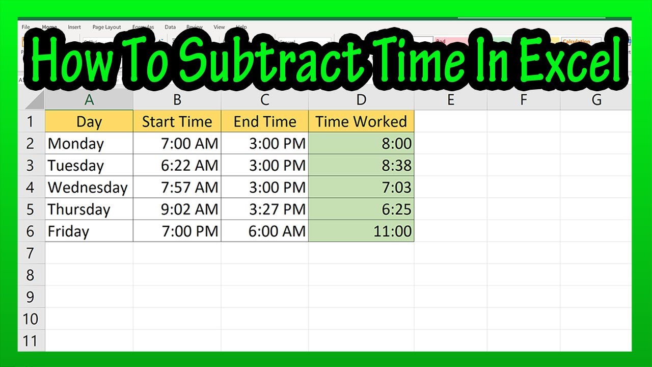
Here is an excel spreadsheet that lists the time worked for a given 5 day period. I will link a video at the end of this video on how to format cells for time values.
As for this video, let’s say that we want to find the times worked each day, and put the results in column D.
To do this, we first have to format the cells, in column D, cells D2 through cell D6, where the results are going to go.
We start by left clicking and holding on the first cell we need to format, in this case cell D2, so it is highlighted. Next, we are going to hold and drag down to the last cell, cell D6, and then release the click and hold. You can see these cells are now highlighted.
Next, we are going to left click once, anywhere in the highlighted cells area, and a drop down box will appear. We are going to go down to format cells… and left click on it.
Now, this pop up box appears, and under the number tab, we are going to go down to Time, and left click on it. Now, another box appears giving some options on how we want the time formatted. We are going to go down to the time format that has the hour, colon, and the minutes, this 13:30 here. We will left click on it, and then click on OK at the bottom of the box.
Now, we are ready to do the calculations. For the first day, Monday, we start by left clicking on cell D2, so it is highlighted, then we type in the equals sign, next we left click on the cell we are subtracting from, in this case the end time, cell C2, then we type in a minus sign, next, we left click on the cell we are subtracting, in this case the start time, cell B2. And we finish by hitting the enter key, and we get our answer of 8 hours.
And that is how to subtract times in excel. To finish the table off, we can do this quick, by left clicking on the cell we just completed, cell D2, so it is highlighted, and we are going to move the cursor down to the bottom right hand corner of the cell, and the plus sign will turn black. From here, we will left click and hold and drag down to the last cell, cell D6. And then we will release the click and hold, and we have our daily time worked filled in, with one exception, Friday has all of these pound signs. That is because the time worked goes past midnight, so this has to be handled a little differently.
I will cover this in the next excel video, and I will link that video at the end of this video.
Chapters/Timestamps
0:00 Set up/Intro
0:16 First format the cells for time accumulation values
1:13 Doing the calculations for time accumulation
1:40 Doing the calculations for multiple cells at one time
Комментарии
 0:05:31
 0:01:31
 0:05:47
 0:08:24
 0:00:16
 0:00:57
 0:00:13
 0:02:31
 0:23:20
 0:00:10
 0:05:33
 0:03:10
 0:08:05
 0:00:53
 0:05:07
 0:06:34
 0:08:11
 0:04:05
 0:00:18
 0:03:25
 0:04:53
 0:03:57
 0:02:59
 0:14:06