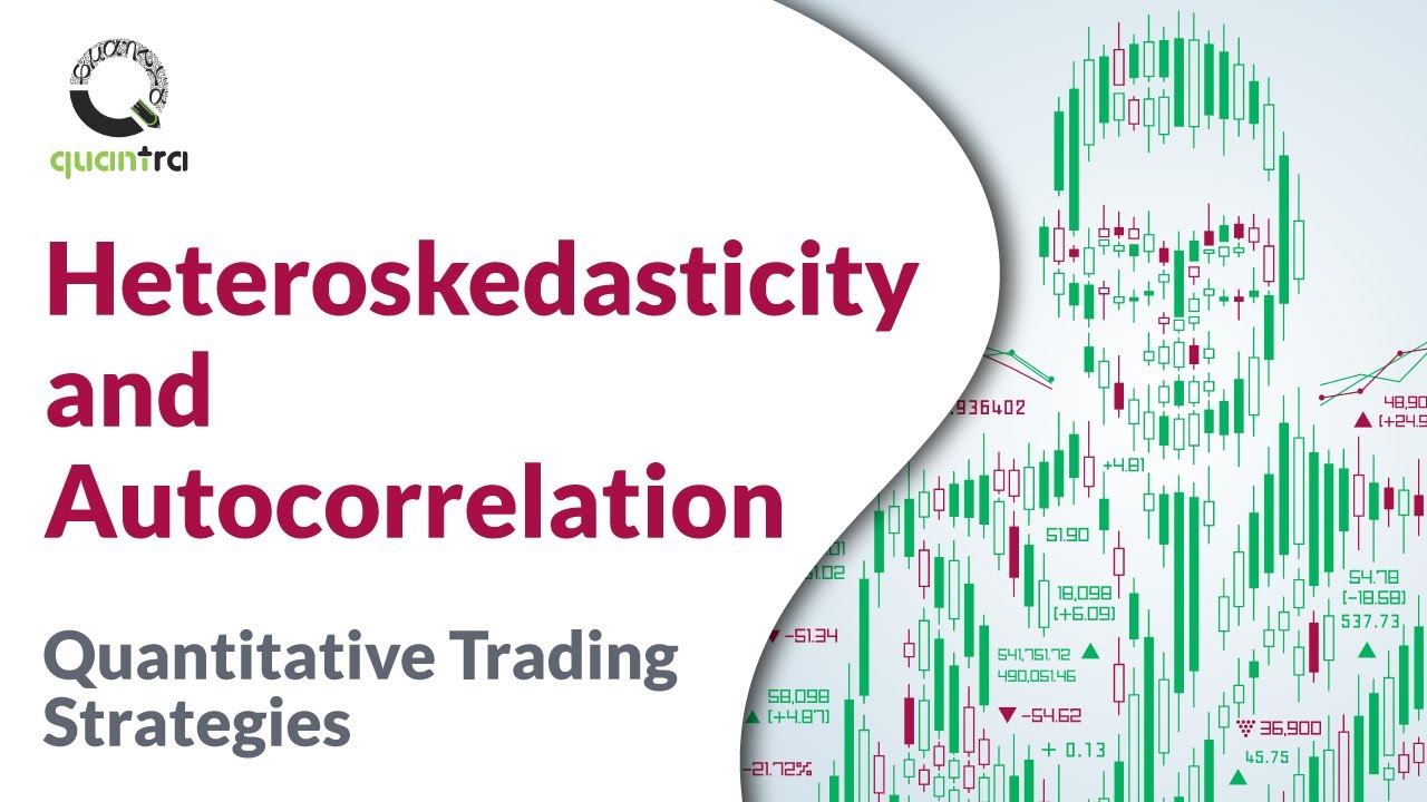
Heteroskedasticity and Autocorrelation | Quantitative Trading Strategies and Models | Quantra Course

Video from the course Quantitative Trading Strategies and Models
***START FOR FREE***

Welcome to this video lecture! The objective of this video lecture, is to cover the required concepts for understanding the ARIMA and GARCH models. The concepts that we will learn in this video lecture are as follows,
1.Heteroskedasticity,
2.Serial Correlation or Autocorrelation.
Let us begin with heteroskedasticity. If we correctly recall, one of the assumptions of linear regression is that the variance of its errors is constant across all the observations of the financial data. In other words, we can say that the errors are homoskedastic.
This graph shows the values of the dependent and independent variables and a fitted regression line with homoskedastic errors. These errors or residuals are the vertical lines between the plotted or actual points and the fitted regression line or
forecasted points.
However, in heteroskedasticity errors are not constant. You may look at the difference between the two graphs. Unconditional heteroskedasticity occurs when the variance in errors is not correlated with independent variables or in other words error variance does not systematically increase or decrease with the changes in the values of independent variables.
Though this violates the assumption, it is not statistically significant and causes no major problems while forecasting variables using regression analysis. On the other hand, conditional heteroskedasticity is what causes problems in forecasting since it is statistically significant.
It occurs when the variance in error is correlated with independent variable. In this graph as the value of the independent variable increases the variance in the error term also increases. The highlighted area is that of low residual variance and this one is that of high residual variance.
Fortunately, there are many software packages that can detect heteroskedasticity. Breusch Pagan test is widely used in finance research owing to its generality. Correcting heteroskedasticity is also common using robust standard errors or generalised least squares which help to eliminate heteroskedasticity.
The next term we need to understand is serial correlation. Serial correlation or autocorrelation occurs when the regression errors are correlated with one another. Understand the difference between conditional heteroskedasticity where the errors are correlated with the value of iindependent variables and autocorrelation where the errors being correlated amongst themselves.
Positive serial correlation is when a positive error for one observation increases the probability of a positive error for next observation. A negative serial correlation is when a positive error for one observation increases the probability of a negative error for the next observation.
In this figure, the assumption is that of first-order serial correlation or serial correlation between adjacent observations. Serial correlation is potentially a more serious problem than heteroskedasticity. It causes too many Type 1 errors that is rejection of null hypothesis when it is actually true leading to improper investment decisions.
Autocorrelation is detected using a Durbin Watson statistic and corrected by adjusting the standard error of coefficients using Hansen method. It is important to study the terms heteroskedasticity and autocorrelation as financial time series are generally heteroskedastic and autocorrelated when regressed.

Quantra is an online education portal that specializes in Algorithmic and Quantitative trading. Quantra offers various bite-sized, self-paced and interactive courses that are perfect for busy professionals, seeking implementable knowledge in this domain.