How to Create Filter in MS Excel

How to Create Filter in MS Excel?

In this tutorial, we dive into the essentials of creating and clearing filters to efficiently manage your data, whether you're handling a large dataset or simplifying everyday tasks. Perfect for both beginners and seasoned users looking to refine their Excel skills.

Steps to Create Filter in MS Excel:
1. Prepare Your Data:
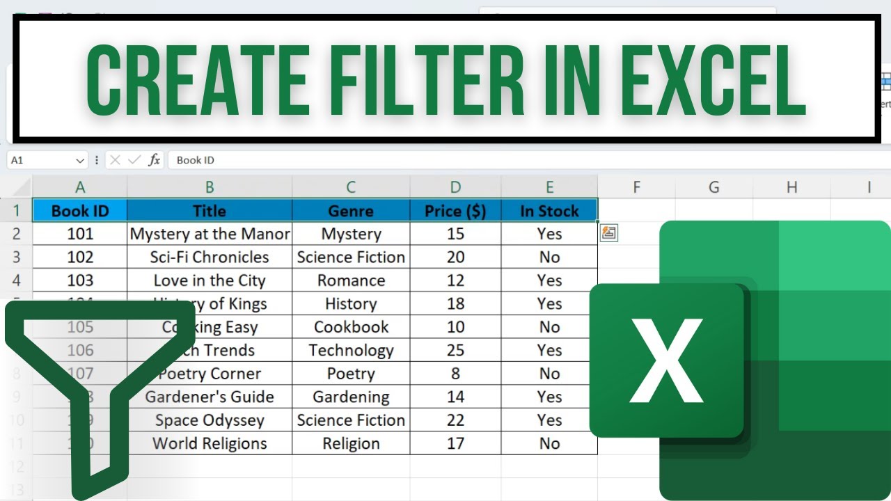
- Ensure your dataset includes headers. For example, 'Book ID', 'Title', 'Genre', 'Price', and 'In Stock'.
- Select the headers.

2. Enable Filtering:
- Navigate to the 'Data' tab.
- Click on the 'Filter' button in the 'Sort & Filter' group.
- Dropdown arrows will appear in each header cell.

3. Apply a Filter:
- Click the dropdown arrow next to a column header (e.g., 'In Stock').
- Deselect all options except for 'Yes' to filter for available books.
- Click 'OK' to apply the filter. Only rows meeting the filter criteria will be displayed.

4. Apply Multiple Filters:
- To add another filter, click the dropdown for 'Genre'.
- Deselect all and then select 'Science Fiction'.
- Click 'OK'. Now, the data shows only 'Science Fiction' books that are available.

Clearing Filters:
1. Clear All Filters:
- Go to the 'Data' tab.
- Click 'Clear' in the 'Sort & Filter' group to remove all applied filters and display all data.

2. Clear Filters Individually:
- Click the funnel icon in the filtered column header.
- Select 'Clear Filter from [Column Name]' to remove the filter from that specific column.

3. Remove Filter Controls:
- To completely remove filtering, select the dataset headers.
- Click the 'Filter' button again in the 'Data' tab. This will remove all filter dropdowns.

- If this tutorial was helpful, please give it a thumbs up, subscribe to WebWise channel for more easy-to-follow tech tutorials, and leave any questions or suggestions in the comments below.