Tutorial 12 - Data-enabled groundwater modeling with 'remote' no-flow boundary conditions.

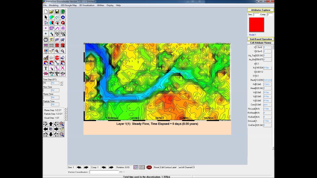
This video illustrates the use of IGW to create a Google Maps-based “one-click” data-enabled model. The modeler uses Google Maps to zoom and pan to the area to be modeled, and selects and draws a box in the area of interest. In one click, the box drawn in the GIS environment is converted to a model in the IGW environment. This model uses detailed existing datasets, such as Digital Elevation Models, bedrock elevation rasters, and hydraulic conductivity rasters from a massive statewide wells database. The source of water to this model is the statewide groundwater recharge raster, and the sink in this model is the land surface, which acts as a drain. The model is quickly run and compared to available static water level data. The calibration plot shows that while the overall model prediction is consistent with the data, it requires some improvement. One easy method for model calibration is illustrated in this video. Since key model parameters, such as hydraulic conductivity and recharge are obtained from statewide rasters that vary throughout the model domain, these parameters can be easily modified using a multiplication factor. In this video, the recharge and conductivity values are multiplied by a constant throughout the modeling domain. By making global changes to the parameters, the model performance improves, which is seen from the improved model indicators.
The steps to create the model are outlined briefly:
(1) In the Google Map interface, pan and zoom into an area just east of Kalamazoo, Michigan. Pan by click-dragging across the display, and zoom in by double-clicking the left mouse button. To zoom out, double-click the right mouse button.
(2) When the area of interest is centered and completely contained within the display, click on the ‘Capture GE map’ icon to create a map for IGW. Answer yes to the prompt regarding the projection system used in this modeling example. It is not necessary to reduce the resolution by 50% for the area selected.
(3) The map will be automatically opened in the GIS layer explorer. Click on the ‘Draw a rectangle for IGW’ icon and draw a rectangle to define the modeling extent to be used in the IGW main window. By default, the boundaries of the model are assigned as no-flow boundaries as was the case in earlier examples.
(4) Click on the ‘Data enabled modeling…’ icon to create a preliminary model. A prompt will appear to clarify the datasets and key model features used to create the preliminary model. Select ‘Yes’ to proceed, and note that the Google map is automatically imported and set at the basemap.
(5) Discretize the model using a slightly finer grid than would be provided with the default settings
(6) Edit the head display options. Enable zoned (color filled) head display, and run the model
(7) Select the domain polygon in Attributes Explorer, and then return to the GIS interface. Click on the ‘Add new modeling layer’ icon to add wells from the statewide database.
(8) Draw a selection box that is the same size as the model domain (shown as a blue rectangle)
(9) Click on the ‘Data Explore’ icon to import static water levels (SWL) from the drift wells selected in the previous step.
(10) After importing the SWL, leave the ‘Spatial Analysis’ window open and go to ‘Utilities’ - ‘Data Sampling’ - ‘Show Model vs. Obs Sampling at Wellogic …’, then select ‘Averaging in a layer’. Add a 1 stand deviation confidence interval to the plot. Although the overall model prediction is consistent with the data, it requires some improvement.
(11) To improve the calibration, we apply a multiplication factor to the recharge and conductivity rasters. Select the “top” ‘Zone 2’ - the one higher in the project tree along the left side of Attributes Explorer.
• In the ‘Source and Sinks’ tab, check ‘Recharge’ and the ‘Rate’ box just below, then enter a multiplication factor of 1.2
(12) Discretize and run the model
(13) After viewing the calibration plot, it is clear that the calibration can still improve. Again, select the “top” ‘Zone 2’. In the ‘Physical Properties’ tab, check ‘Conductivity’, then enter a multiplication factor of 0.75 in the input box
(14) Discretize and run the model
(15) Note the improvement in the calibration after applying a multiplication factor for both the recharge and conductivity rasters. This is seen qualitatively in the calibration plot and when examining the model calibration indicators

- Hydrosimulatics Inc.