Create a Dynamic Chart Title Sourced from Pivot Table & Slicer

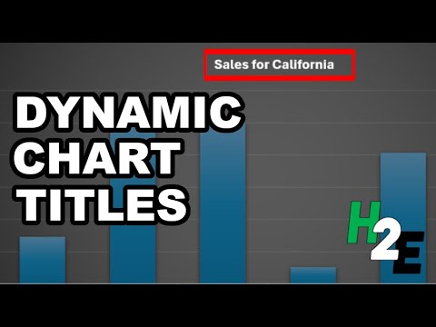
Pivot Tables are one of the best analytical tools in Excel. To enhance and better present the data / information to your audience, you'd need to have a chart to visualizes the data. You may also have a meaningful title, but what if you want to change the Pivot Table? You'd think that you might need to manually change the title to reflect the pivot table chart. Nope! You can use slicers and an additional table to create dynamic text to put into your chart title.

Timestamps
0:00 Intro
0:34 Demo
0:55 Create Table
1:18 Create Pivot Table
1:42 Create Slicer
2:00 Create Chart
2:48 Create 2nd Pivot Table
3:40 TEXTJOIN Formula
4:40 Add Dynamic Text to Chart
5:35 Hide Helper Rows

📝 This description may contain affiliate links and we'll receive a small commission if a purchased is made using the links (but at no additional cost to you). It'll support the channel and so more videos like this can be made. Thanks for your support!

#excel
#msexcel
#dough

[mattstone]

Thank you for the video, it was really clear and helpful

[wayneedmondson]

Nice one Doug! A very handy trick. Thanks for sharing :)) Thumbs up!!

[appetite]

Really good, that has given me some ideas! Thank you

[jdcyh]

How would I add colour to the bars that the slicer has selected?

[CJ-jctn]

Thank you for this video. It was most informative. One question for you: Is there any way to have the dynamic title say "All letters" when you clear the slicer rather than it showing all the letters of the alphabet? I actually have a slightly different use case where I have a slicer of US State names. If I clear the slicer, I'd prefer the title just to say "All States". Thank you

[Yonglee]

But it is not work for pivotchart, data source is power query.