filmov
tv
Python Tutorial : Bootstrap confidence intervals

Показать описание
---
You have now used graphical exploratory data analysis, or EDA, to investigate the active bouts of the zebrafish. I remind you of one of my favorite quotes from John Tukey.
Exploratory data analysis can never be the whole story, but nothing else can serve as a foundation stone--as the first step.
In this course, and throughout your data science endeavors in general, it is important to heed Tukey's advice and start with EDA.
Now that we have done some EDA, let's start progressing toward the whole story.
We saw in the previous exercises that the active bout lengths are roughly Exponentially distributed. The Exponential distribution has a single parameter that describes the characteristic time between arrivals of a Poisson process.
The value of that parameter that best describes the data is computed from the mean of all of the active bout lengths. Thus, the mean computed from the data is the optimal parameter value.
But how confident are we in this value? What if we could somehow measure a collection of inter-incident times again? What would we get for the mean?
We can plot the ECDF of the resampled data, along with the mean inter-incident time computed from this resampled data set. We get a slightly different value than we got from the original data.
We can do this procedure again and again and again and again and again and again.
Each value of the mean inter-incident time is a bootstrap replicate, which is generally a statistic computed from a resampled data set. In this case, that statistic is the mean.
The `dc_stat_think` module has a function to draw bootstrap replicates from a data set. For example, you can use it to draw ten thousand replicates of the mean from a data set.
In looking at the plot of the replicates, shown by the vertical gray lines, we see that the replicates lie somewhere between about 70 and 100 days. This is roughly the bootstrap confidence interval of the mean inter-incident time.
Generally, a p-percent confidence interval can by defined as follows. If we repeated measurements over and over again, p% of the observed values would lie within the p% confidence interval.
Because the bootstrap replicates are simulating measurements over and over again, we can simply take percentiles of the bootstrap replicates to compute the confidence interval.
For the 95% confidence interval, we compute the 2.5th and 97.5th percentiles.
We can do that using Numpy's `percentile()` function. The first argument is an array containing the bootstrap replicates, and the second is a list or tuple with the desired percentiles. We get a 95% confidence interval the spans from 73 to 102 days.
Now that you are refamiliarized with computing optimal parameters and obtaining bootstrap confidence intervals, you can quantify active bout lengths of wild type and mutant fish.
#DataCamp #PythonTutorial #CaseStudiesinStatisticalThinking #StatisticalThinking
Комментарии
 0:03:58
 0:15:39
 0:11:15
 0:09:27
 0:28:33
 0:04:19
 0:10:56
 0:17:03
 0:09:06
 0:06:12
 0:12:51
 0:09:40
 0:25:18
 0:26:24
 0:16:30
 0:00:22
 0:13:52
 0:05:53
 0:20:31
 0:03:48
 0:22:42
 0:04:34
 0:16:30
 0:12:57