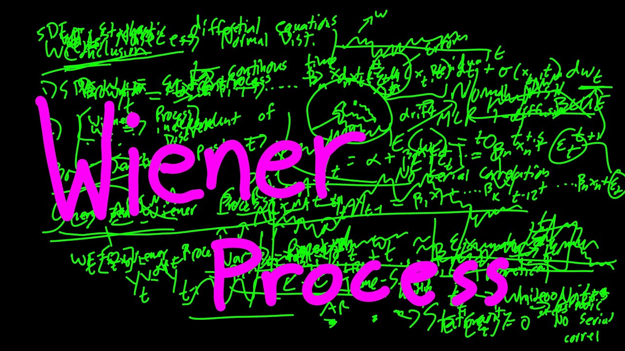
Wiener Process - Statistics Perspective

Quantitative finance can be a confusing area of study and the mix of math, statistics, finance, and programming makes it harder as everyone comes from a different background. In this video I explain the Wiener Process which is also known as Brownian Motion from a statistical model perspective. The residuals of a model in traditional discrete time-series models such as OLS and ARIMA have specific properties which are a zero mean and no serial correlation. These properties are known as White Noise. This white noise can be found in nature as Brownian Motion (Wiener Process). A botanist named Robert Brown discovered this as he watch a particle of pollen float around water.

In continuous time-series (stochastic models) we have a Wiener Process denoted as w(t) at the end of the equation. In many math operations it will cancel out because the mean is zero however the properties of White Noise is what makes the specification of the formulas correct. If it was just ignored and the assumptions not tested, they would be incomplete and often wrong.

Stationarity Introduction:

Stationarity Complexity Explained Using the Mandelbrot

DF and ADF Stationarity Testing

Stationarity in Finance with Applications

Probability, Stationarity, and Failures in Finance

Website:

Support:

Quant t-shirts, mugs, and hoodies:

Connect with me:

[jasdeepsinghgrover]

Thanks for the amazing video.. I was about to start with the book Dynamic Hedging and Statistical Consequences of Fat Tails... This seems a very good general into 🙂

[andresrossi]

The relationship between the Weiner differential component and the error term in a statistical model is brilliant. Seems like they have different roles but it's conceptually the exact same thing. Good content Dimitri

[igorbaglay]

I, too, wish this was taught more approachable for people with statistical background. The "mean and nasty" teacher story at 16:20 rings a bell.. :) For me, the key intuition with that SDE was that it was for a Geometric Brownian Motion, meaning that it was a multiplicative process (unlike ARIMA which is inherently additive). And so the the distribution was log-normal, which is the "normal" for the multiplicative domain. I.e. Gibrat's law being similar to CLT. I wish that connection was made earlier, then the Black Scholes derivation would be easier to understand.

[maximoppitz]

Thank you, I’m an mfe student and I think a lot of programs are lacking on bringing time series and stochastic calculus together! Thank you for giving some intuition on how these things relate. Have a good one!

[armanmuslimov]

Awesome! Dmitri, please keep doing this kind of videos about different areas of quant finance topics and your perspective on them. Examples of practical application, associated challenges, common mistakes and consequences could also be great. Thanks for the interesting content!

[raphaeltaieb]

This kind of videos are amazing. It would be great to have more videos like this

[dovi]

As a Financial Mathematics major, your professor probably used quadratic variation to show that terms (dt^2) were 0. Taylor Series and quadratic variation are the bedrocks to Ito formula, so it makes sense that your professor used to to prove the Black-Scholes PDE.

[Ligma]

Dimitri I'm researching about the topic of my dissertation. What's your take on SABR model? Are they used in the industry now? What other stochastic volatility/risk models do you recommend? And what are the other areas or topics that have "momentum" now?
Sorry I'm so confused... and you're the only real quant that I know.

[martinsanchez-hwfi]

Thank you for the video, but there are some inaccuracies. The W_t is not independent of the past. It is a Martingale and a Markov process. It is only non overlaping increments of W_t which are independent of each other. There are other things, but that was the one worth mentioning

[daanialahmad]

Dear Dimitri,

Thank you so much for such a beautiful video

[Ligma]

Dimitri what is the best method for making data stationary? We use log-transformation and simple differencing for our projects, I was wondering if it is this simple in the industry too.
...and brilliant video. Thanks

[MilkTea-sxgd]

This was absolutely amazing, thank you

[Eta_Carinae__]

I think wrt Brownian motion, that it was the motion of a water droplet very close to boiling on a hot plate. I think it was also Einstein of all people who first captured that motion with equations, if my history is right.

I just realised that SDEs are distinct from normal DEs in that the notion of a derivative implies smoothness when zoomed into the function, but SDEs do not. I have a feeling that derivatives of the itô process would look basically the same as the itô process - in that they'd diffuse and drift in like.

Do you have a proof of dx_t in the itô process? I take it that dx_t means the same thing as it does in bog standard calculus.

[artlenski]

White means the spectrum is flat in other words it describes correlation properties of a process. Gaussian means that increments/changes are distributed according to Gaussian distribution. Hence a process could white and not gaussian, or gaussian and not white. AGWN: additive gaussian white noise is a popular choice as it mimics the effect of many random processes that occur in nature.

[small]

I think this is brilliant if understood from an intuitive perspective, however, stochastic calculus is pure mathematics, hence absolute - it is based on definitions. It cannot be reduced to intuition.

[diviyampat]

hey, have watched you watched Quantpy youtube channel it looks interesting and it would be interesting listening to your opinions😇

[kolonniki]

You’re going to talk about the wiener process and not make a single joke about the name? 😂
Very interesting video though!

[devez]

Would you recommend the book “Introduction to Time Series and Forecasting”, Peter J. Brockwell
Richard A. Davis?