filmov
tv
video 10.2. post hoc tests & family-wise error
Показать описание
closed captioning text:
If you do an ANOVA and it is statistically significant, if you reject the null hypothesis, then you have to do a post hoc test to tell which of the many means are different from one another, but you might wonder why do you even have to do an ANOVA at all. Why not just do t-tests that compare each of the groups? So I will briefly explain that before I introduce post hoc tests.
So the reason you can not just compare all the different means... so if we have intro, research design, and statistics, we have those those three different samples. If we do t-tests, the first two tests would be comparing these two. That would have an alpha equal to .05. Then if we do comparison of these two, that would have a different alpha equal to .05. So we have to compare 1 and 2, 2 and 3, and then also 1 and 3. Now I would have at alpha of .05. So we would have to do three statistical tests, instead of one. If we do three statistical tests instead of one, then our alpha is not going to be .05 anymore. So if you do just one test, alpha is .05, but if you have three means, and you have to do three comparisons, then the probability of a type 1 error with three different means, the alpha turns into .143. You might think it should be .05 times 3, but what happens is that some of the times you would have a false positive on two different tests or even all three. That is why this is not .15.
So this problem of inflated alpha here is called "family-wise error rate." So your false positives are higher if you do more comparisons. So the family-wise error rate is the probability of a type 1 error for a set (that is, a "family") of statistical tests. This is why when we are comparing three different means, these for example, we do an ANOVA first rather than doing three t-tests. As you will see in a little bit, the post hoc test is actually, basically, doing three different t tests, comparing each of these pairwise. It is slightly modified though.
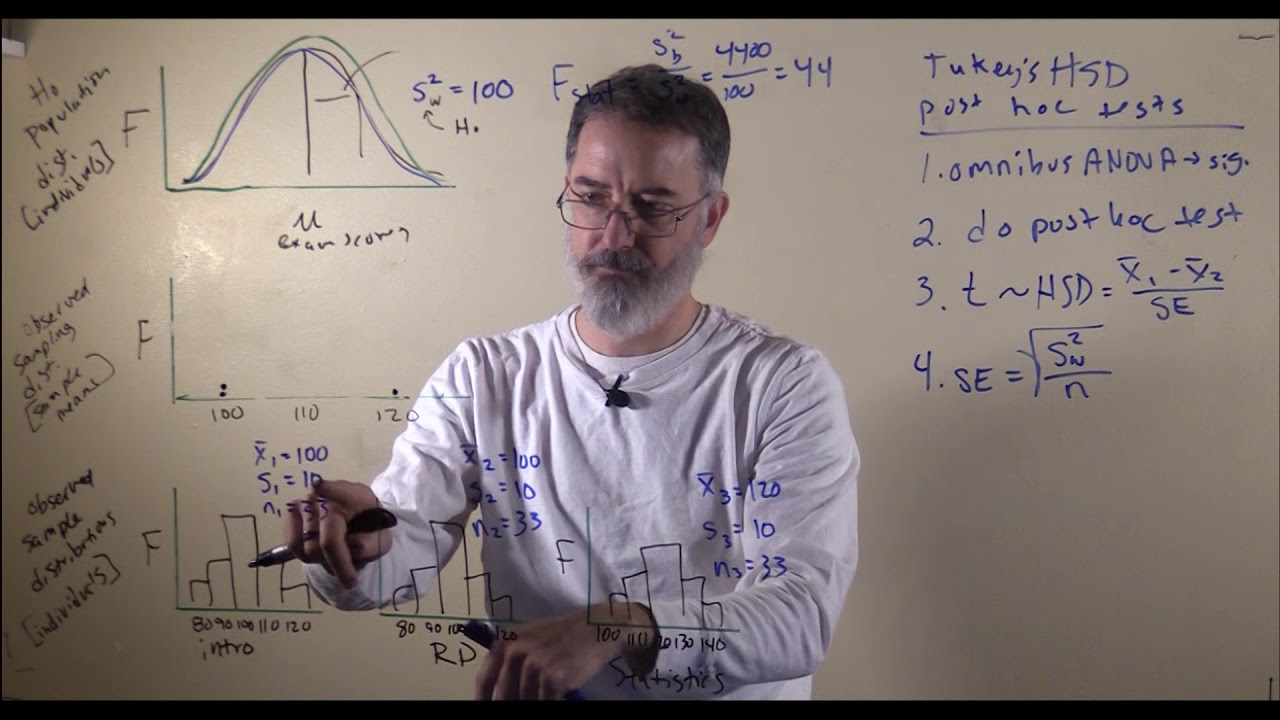
So when you are doing ANOVAs and you are comparing three or more means, the first thing that you will want to do is the regular ANOVA that we talked about in the previous video. That is called the "omnibus ANOVA" because this one analysis of variance compares all three means at the same time. Only if you reject the null hypothesis, if your p-value is less than alpha, if your test statistic is more extreme than your critical value, only then you can do the post hoc tests, which will tell you which means are different from one another. Post hoc means "after the fact" or "after this", so after the overall ANOVA is significant, then you will do those pairwise comparisons. By using this strategy, it keeps the overall alpha rate to .05 like you want it to be.
So there are a lot of different post hoc tests available for researchers to use. I am gonna stick with Tukey's honestly significant difference test, because it is very similar to a t-test, and it is commonly used as well. So it is also known as Tukey's HSD, honestly significant difference test. So Tukey's HSD post hoc test. So that is what we will do next here. So recall the first thing is the omnibus ANOVA has to be statistically significant. That term "statistically significant" means that you have rejected the null hypothesis. So you only do these post hoc test if that is the case. Then so if that is significant, you do your post hoc test. Tukey's is a modified t-test. That is the easiest way to think about it: a modified independent-groups t-test.
So one reason it is different than the t-test is with a t-test you only had two different groups, but with having done an ANOVA, we have three different groups. So we have three different estimates of the population's variance, and we are going to use all of those for our t-test. So for our standard error, what we are gonna do for this, is use the variance-within divided, by the sample size. Remember this will work only if your sample sizes are all the same, which they are for us. Of course, it has got to be the square root. This is the population's variance estimate, and we want to turn it into a standard error. We need to divide it by the sample size, and then take the square root. Another way it is a little bit different than the t-test, is there is a modified critical values table. This will keep our alpha at .05 or so.
[closed captioning continued in the comments]
If you do an ANOVA and it is statistically significant, if you reject the null hypothesis, then you have to do a post hoc test to tell which of the many means are different from one another, but you might wonder why do you even have to do an ANOVA at all. Why not just do t-tests that compare each of the groups? So I will briefly explain that before I introduce post hoc tests.
So the reason you can not just compare all the different means... so if we have intro, research design, and statistics, we have those those three different samples. If we do t-tests, the first two tests would be comparing these two. That would have an alpha equal to .05. Then if we do comparison of these two, that would have a different alpha equal to .05. So we have to compare 1 and 2, 2 and 3, and then also 1 and 3. Now I would have at alpha of .05. So we would have to do three statistical tests, instead of one. If we do three statistical tests instead of one, then our alpha is not going to be .05 anymore. So if you do just one test, alpha is .05, but if you have three means, and you have to do three comparisons, then the probability of a type 1 error with three different means, the alpha turns into .143. You might think it should be .05 times 3, but what happens is that some of the times you would have a false positive on two different tests or even all three. That is why this is not .15.
So this problem of inflated alpha here is called "family-wise error rate." So your false positives are higher if you do more comparisons. So the family-wise error rate is the probability of a type 1 error for a set (that is, a "family") of statistical tests. This is why when we are comparing three different means, these for example, we do an ANOVA first rather than doing three t-tests. As you will see in a little bit, the post hoc test is actually, basically, doing three different t tests, comparing each of these pairwise. It is slightly modified though.
So when you are doing ANOVAs and you are comparing three or more means, the first thing that you will want to do is the regular ANOVA that we talked about in the previous video. That is called the "omnibus ANOVA" because this one analysis of variance compares all three means at the same time. Only if you reject the null hypothesis, if your p-value is less than alpha, if your test statistic is more extreme than your critical value, only then you can do the post hoc tests, which will tell you which means are different from one another. Post hoc means "after the fact" or "after this", so after the overall ANOVA is significant, then you will do those pairwise comparisons. By using this strategy, it keeps the overall alpha rate to .05 like you want it to be.
So there are a lot of different post hoc tests available for researchers to use. I am gonna stick with Tukey's honestly significant difference test, because it is very similar to a t-test, and it is commonly used as well. So it is also known as Tukey's HSD, honestly significant difference test. So Tukey's HSD post hoc test. So that is what we will do next here. So recall the first thing is the omnibus ANOVA has to be statistically significant. That term "statistically significant" means that you have rejected the null hypothesis. So you only do these post hoc test if that is the case. Then so if that is significant, you do your post hoc test. Tukey's is a modified t-test. That is the easiest way to think about it: a modified independent-groups t-test.
So one reason it is different than the t-test is with a t-test you only had two different groups, but with having done an ANOVA, we have three different groups. So we have three different estimates of the population's variance, and we are going to use all of those for our t-test. So for our standard error, what we are gonna do for this, is use the variance-within divided, by the sample size. Remember this will work only if your sample sizes are all the same, which they are for us. Of course, it has got to be the square root. This is the population's variance estimate, and we want to turn it into a standard error. We need to divide it by the sample size, and then take the square root. Another way it is a little bit different than the t-test, is there is a modified critical values table. This will keep our alpha at .05 or so.
[closed captioning continued in the comments]
 0:12:24
ANOVA 2: Post Hoc Tests in One-Way ANOVA
 0:11:12
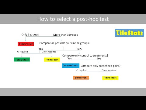
How to select a post hoc test
 0:05:52
PSY 230 Video 12 9 Post Hoc Tests
 0:06:10
Post-Hoc Tests for One-Way ANOVA
 0:21:31
Parametric Tests : ANOVA - Analysis of Variance Statistical Test Types One Way Two Way Post Hoc Test
 0:43:56
Permutational ANOVA: Posthoc Tests
 0:10:28
Selecting a Post Hoc Test after ANOVA in SPSS
 0:08:17
How To... Perform an ANOVA Post-Hoc Test in R #90
 0:05:42
HIMALAYAN SALT BENEFITS: 20 Reasons to Make the Switch!
 0:09:04
Student-Newman-Keuls Post-Hoc Test (By Hand)
 0:14:21
ANOVA with Bonferroni Correction (Bonferroni Post Hoc Test) in SPSS
 0:15:51
One-way ANOVA and Tukey's post hoc tests using SPSS
 0:16:16
SPSS (9): Mean Comparison Tests | T-tests, ANOVA & Post-Hoc tests
 0:36:00
Lec 25, Post Hoc Analysis(Tukey’s test)
 0:12:52
Foundations of ANOVA – Variance Between and Within (12-2)
 0:10:20
Post hoc test | Fisher's LSD – explained
 0:10:21
One-way ANOVA & Post-Hoc Analysis in Excel
 0:08:39
Post hoc test | Bonferroni - explained
 0:12:52
One-way ANOVA and Tukey's post hoc tests via two routes in SPSS (June 2020)
 0:01:07
SPSS ANOVA Post hoc tests - Easy tutorial by StatisticalGP
 0:29:17
Duncan Multiple Range Test (DMRT) with Compact Letter Display
 0:04:30
JASP repeated measures ANOVA and post hoc tests
 0:10:00
J6 - Two-way ANOVA: post-hoc tests
 0:14:10
Three Way ANOVA Post hoc test in SPSS
Комментарии