filmov
tv
Using Mathematica for ODEs, Part 10. More modularity in Mathematica programming.
Показать описание
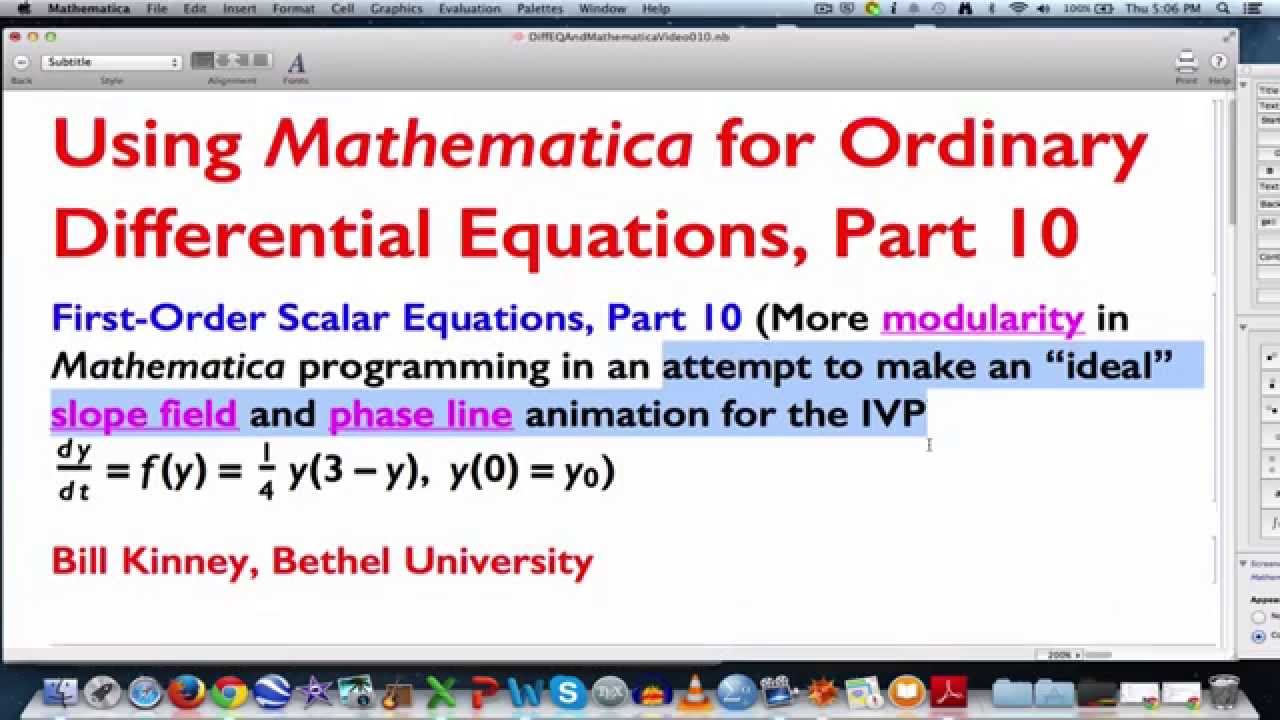
Using Mathematica for ODEs, Part 10. More modularity in Mathematica programming in an attempt to make an "ideal" slope field and phase line animation for the IVP dy/dt = f(y) = y*(3-y)/4, y(0) = y0.
AMAZON ASSOCIATE
As an Amazon Associate I earn from qualifying purchases.
 0:10:53
Using Mathematica for ODEs, Part 5 (Use Manipulate to see solutions change as parameters change)
 0:10:29
Using Mathematica for ODEs, Part 1 (Use DSolve and Plot for a pure antiderivative problem)
 0:13:17
Using Mathematica for ODEs, Part 10. More modularity in Mathematica programming.
 0:14:08
Using Mathematica for ODEs, Part 7...a smorgasbord of misc Mma and math subtleties
 0:12:32
Using Mathematica for ODEs, Part 4 (use DSolve, Plot, VectorPlot, Show, Simplify, Solve, & Apart...
 0:11:19
Using Mathematica for ODEs, Part 2 (Use VectorPlot and Show for a pure antiderivative problem)
 0:13:04
Using Mathematica for ODEs, Part 6 (using DSolveValue, Manipulate, VectorPlot, pure functions)
 0:09:14
Solving Differential Equations(ODEs) in Mathematica | Tutorial -11
 0:14:11
Using Mathematica for ODEs, Part 8. Review slope fields for autonomous eqs. Phase lines.
 0:05:08
Numerically Solve ODEs with Mathematica 2
 0:13:03
Using Mathematica for ODEs, Part 9. Equilibrium points (sinks & sources) on phase line. Modulari...
 0:10:32
Using Mathematica for ODEs, Part 3 (DSolve, VectorPlot...make a Slope Field for an Autonomous Eqn)
 0:06:02
Numerically Solve ODEs with Mathematica 1
 0:16:59
Solving ODEs Analytically Using Mathematica
 1:08:26
Mathematica for ODEs & Slope Fields: DSolve, DSolveValue, VectorPlot, Plot, ContourPlot, Manipul...
 0:05:29
Two different ways to solve Partial differential equations ||(Mathematica tutorials-08)
 0:35:44
Lecture 12 - Solving Ordinary Differential Equations in Mathematica
 0:48:14
Lecture 14 - Implicit methods for ODEs (Hermite integration) in Mathematica
 0:05:42
How to solve first order coupled ODEs: Mathematica
 0:07:56
Slope Fields & Solutions with DSolve on Mathematica for Nonautonomous Differential Equation Exam...
 0:05:37
Solving Differential Equations in Mathematica with Boundary Conditions Given.
 0:02:01
Mathematica: Formulate and solve a system of linear, first-order ODEs in Mathematica
 0:02:41
Mathematica: NDSolve stiff system of ODEs
 0:06:36
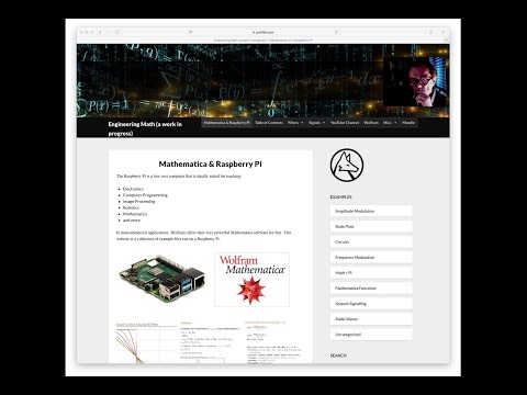
Mathematica & Raspberry Pi - DSolve and 1st order ODEs
Комментарии