Phase Line Examples, Linearization Theorem (Sinks & Sources), Mathematica, First Bifurcation Example

(a.k.a. Differential Equations with Linear Algebra, Lecture 9A, a.k.a. Continuous and Discrete Dynamical Systems, Lecture 9A. #differentialequations).

(0:00) Many examples of phase lines in this lecture
(0:41) Example 1: dy/dt = f(y) = 3y - y^2 = y(3 - y) (Quadratic right-hand side function)
(2:57) Slope field can be drawn from the graph of f(y)
(4:55) The equilibrium solutions are y = 0 and y = 3
(5:25) The Phase Line with a source at y = 0 and sink at y = 3
(7:12) Nodes can occur as well
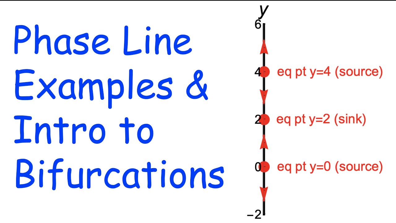
(7:45) Example 2: dy/dt = f(y) = y(y-2)(y-4) = y^3 - 6y^2 + 8y (Cubic RHS function)
(8:35) Graph f(y)
(10:55) The slope field
(11:30) The phase line with sources at y = 0 and y = 4 and a sink at y = 2
(11:58) Mathematica for Example 1
(15:20) Animated phase line for Example 1
(16:35) Mathematica for Example 2 (including NDSolveValue)
(19:09) Idea of Linearization Theorem for Example 2
(22:15) Example 3: dy/dt = f(y) = y(y-2)^2 (Cubic RHS with a double root)
(22:41) Graph just touches the axis at the double root y = 2
(23:10) Phase line has a node at y = 2
(24:36) Mathematica
(26:46) Example 4: dy/dt = f(y) = y^3 (Cubic RHS with a triple root)
(27:18) y = 0 is a “weak” source (Linearization Theorem does not apply)
(28:19) Mathematica
(31:24) Example 5: dy/dt = f(y) = cos(y)
(32:32) There are infinitely many equilibrium points on the phase line
(33:28) Mathematica
(35:00) Example 6 (Bifurcation example): dy/dt = f(y) = y^2 + mu
(36:16) How does the phase line change as mu changes?
(37:15) Draw the graphs of f(y) as mu changes
(38:43) Draw the phase lines as mu varies
(39:54) A bifurcation occurs at mu = 0

AMAZON ASSOCIATE
As an Amazon Associate I earn from qualifying purchases.

[georgesadler]

Professor Kinney, thank you for an exceptional video/lecture on the Phase Line Examples, Linearization Theorem and using Mathematica to analyze complex problems. Ordinary Differential Equations is used to study complex systems and nature on planet earth. Mathematica, MATLAB and Maple are all used to study/analyze problems in Differential Equations.