Change the colours of a Pie Chart to represent the data FIgures using VBA

Hi Guys,

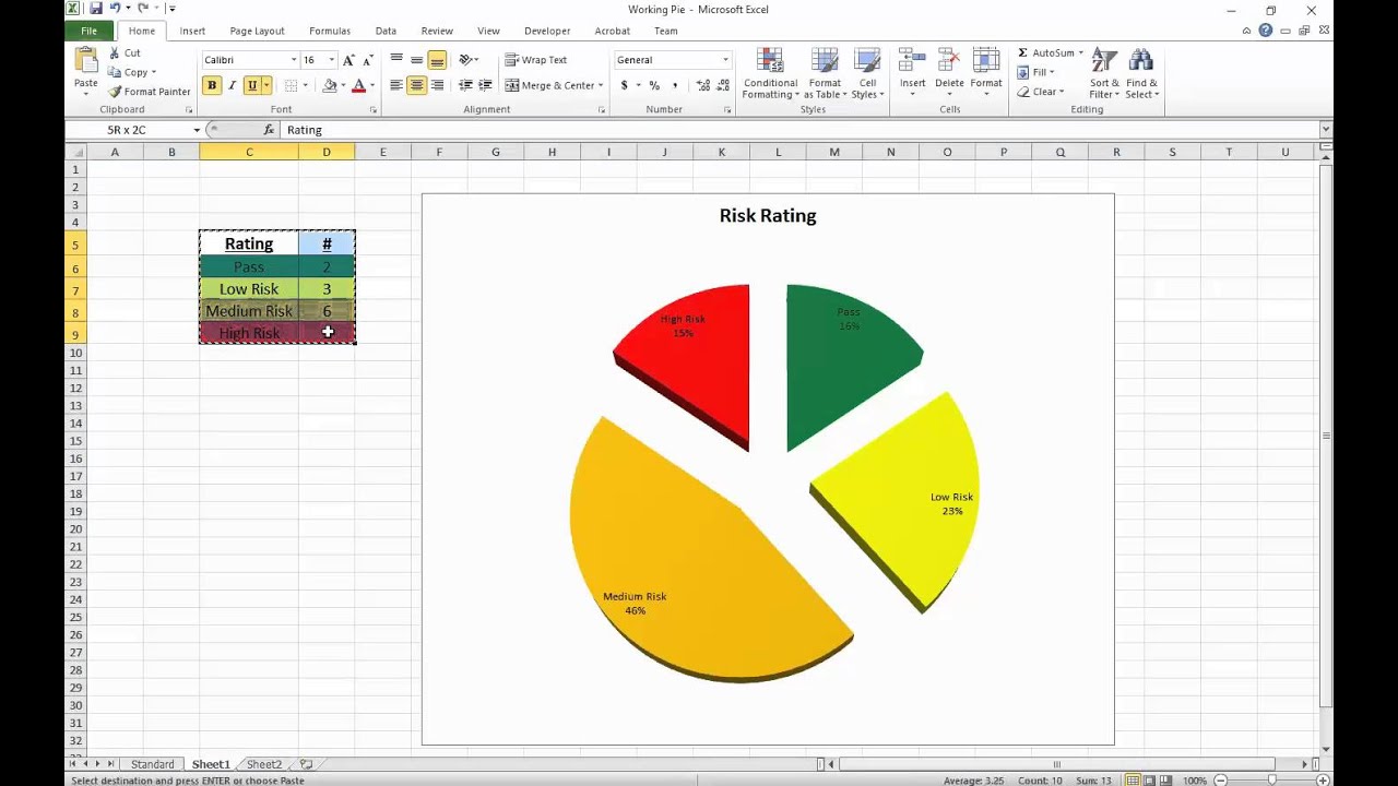
In this quick tutorial we are going to go through making a pie chart in Microsoft Excel show the colours that represent the data that they are displaying.

If you have a table that shows data for low risk (green), Medium Risk (orange) and high risk (red); you may wish to show the pie chart in the same colours as your table.

Excel can't do this as a standard, but with a little bit of VB code, we can get it to work.

Step One: Once you have your table of data and your pie chart. Press ALT and F11 to load the Visual Basics Editor.

Step Two: On the left you will see sheet 1, sheet 2 etc. Double click onto the sheet that you have the Pie Chart on.

Step Three: Paste the code from the video.

Step Four: Save the code and the spreadsheet. Close and reload.
Now it should be working.

PLEASE NOTE THAT THE DATA TABLE MUST CONTAIN THE COLOURS THAT YOU WISH TO BE DISPLAYED IN THE PIE CHART.

[zakirdatey]

How can I have a mouseover event when the mouse is hovering over the pie chart slice, the slice show shadow and color change. Please advice

[adattbanajr]

Hi. Blessed Day. I am working on 2013 and it is not working. Can you pls help me...Thanks

[suravidas]

sir can u please uplaod the code soon. its urgent because i need to sumbit my research project and not able to change the color according to my data color.

[adiyagama]

I am using excel 2016, it does not work for me, can you please help

[valentincontilde]

Guys, I think I just found out why this doesn't work for the most part of us, I tried, tried AND found out this trick:


Do the same steps shown in the video [Excel, alt+F11, etc] but DON'T COPY his code, copy instead this: [CREDITS TO MrMatanay in an older comment here below]




Sub ColorPies()
Dim cht As ChartObject
Dim i As Integer
Dim vntValues As Variant
Dim s As String
Dim myseries As Series

For Each cht In ActiveSheet.ChartObjects
For Each myseries In cht.Chart.SeriesCollection

If myseries.ChartType <> xlPie Then GoTo SkipNotPie
s = Split(myseries.Formula, ", ")(2)
vntValues = myseries.Values

For i = 1 To UBound(vntValues)
=
Next i
SkipNotPie:
Next myseries
Next cht
End Sub


Don't close Excel window, it's not necessary.


Ok, you know the rest, but when you come back to the sheet 2 you have to go where says DEVELOPER in the upper screen side or wherever the option of Macros is... you click there and then you simply click EXECUTE and voilà there is it, you have applied the command you "invented" in THAT sheet.


Buena suerte.


Pd: Another thing is that this dude doesn't clarify about the saving specifications, when you are about to save the file, you have to choose the excel format which holds Macros, Don't panic, it explitcitly says that. Then you save it and the file logo appears with an exclamation mark like that on this dude's video


De nada

[alextompkins]

Hi! Would you mind pasting the code here? Thanks :)

[martina]

I tried copying the code but several "sentences" appear to have errors and appear in three