Locate and Change Excel Pivot Table Data Source

After you create a pivot table, you might add or change records in the source data. Sometimes the pivot table doesn't update correctly, to show the new data.

In this video, you'll see how to locate the pivot table data source, and adjust its size.

You'll also see how to create a dynamic data source that will adjust size automatically.

Visit this page to download the sample file for this video.

Video Timeline

00:00 The Orders Pivot Table
00:21 Manually Check the Numbers
00:33 Find the Source Data
01:08 Change PivotTable Data Source Window
01:27 Fix the Data Source Range
01:57 Create a Dynamic Source
02:48 Create a Named Table
04:22 Use Dynamic Source for Pivot Table
04:56 Test the Dynamic Source
05:31 Conclusion
05:45 Get the Sample File

Instructor: Debra Dalgleish, Contextures Inc.
#ContexturesExcelTips

Video Transcript - Abridged

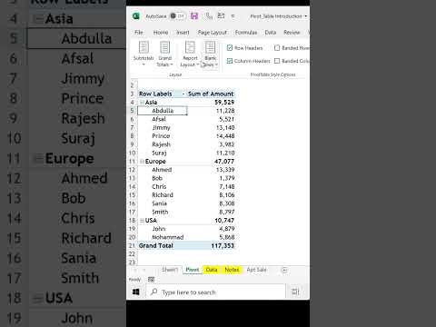
In this video, you'll see how to find the source data for a pivot table and fix that source data, if there's a problem getting the new or changed data that you've entered. In this pivot table, I'm showing orders. One of the products we sell is paper. I entered a new order, and it's not showing up here.

If I refresh, it's not picking up that new record. I'm going to find the source data and see if there's a problem.

To find the source data, select a cell in the pivot table. On the Ribbon, under Pivot Table Tools, click Analyze.

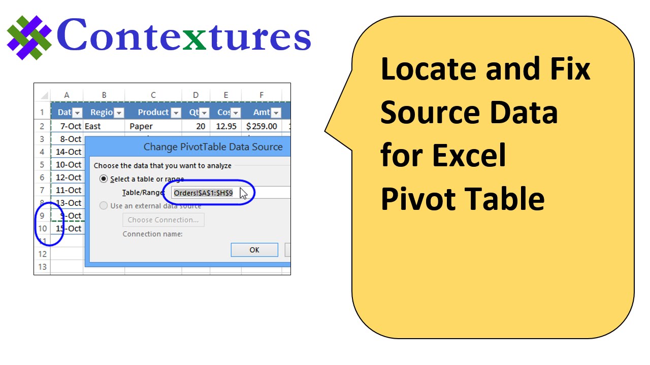
Click here, and here's the Change Data Source. That opens up the Change PivotTable Data Source window.

It's showing that there's a range selected, and I can see moving lines in the background, and one row is not included.

It stops at row 9 and the new record is row 10.

To change this and fix the problem, I can adjust the range that's included here. Back space, and type 10, instead of 9.

Or I can select and delete it. Then on the worksheet, select the range that I want to use. Click OK, and the pivot table shows the new data.

You could continue to adjust that range as you add new rows to the data source. But a better solution is to create a dynamic source for your pivot table, which will adjust automatically, if you add new records.

It's easy to do that, in Excel 2007 or later. Go back to the Orders sheet.

This is just a list typed on the worksheet. We've got column headings and a row for each order, but if I look on the ribbon, there's no Table tab at the top.

We're going to create a named table. To create the table, select a cell in your list and on the Ribbon click Insert, Table.

It does a good job of detecting the range, but if necessary, you can adjust what's typed in here.

Be sure to check My Table Has Headers, then click OK.

You'll get a formatted table. Click on one cell.

To change the formatting that it puts on the table, go to the Design tab, under the Table tab, and select something else.

The next thing you should do is change the name of the table. It will give a default name that ends with a number.

Just select that and I'm going to call this tbl, for table, tblOrders, and press Enter.

So now we have a table name, and I can see that name, if I go to the Formulas tab, Name Manager.

And there's a list of all the names in this workbook. So it makes it easy to spot this, if you have several tables in your workbook.

I'll close this, and the next step will be to use our name, so going back to the Table Tools, we're going to use this name, tblOrders, as our source for the pivot table.

I'm going to just click in here, and then Ctrl+ C to copy that name.

I'll go back to my pivot table now. And then with a cell selected in the pivot table, I'll go back to the Analyze tab, click Change Data Source, and here's the current data source.

I'm going to use Ctrl+ V to paste what I copied as the table name. So it's now going to use this dynamic range which will adjust as we add new records.

Click OK, and nothing looks different here, but I'm going to go and add another order.

Just copy what we have above, by using Ctrl and the double quote. I'll put in 100, so now we should see 320, where we had 220 before.

Going back to Pivot Sales, it still says 220. I'll refresh, and now we've got 320.

So I didn't have to adjust the range of the pivot table source data. That adjusted automatically, because it's a named table.

So if your pivot table data will change frequently, make sure you use a dynamic source, like a named Excel table, and it will adjust as you add or delete records.

[radders]

Thank you for this video, i searched for hours to make my table dynamic and this has helped within 5 minutes.

[jennifermacgregor]

Super clear, much appreciated! I like the zooming and extra graphics to be able to follow what you do on the screen. Thank you!

[Kelveron]

Excellent. That was very clearly and nicely explained, at the right pace. Thank you so much.

[surferdude]

Found exactly what I need by the 3mn mark. Thank you!

[senpai.]

Thank you! I found this very useful. I love your videos and appreciate your efforts. I find them very informative and practical.

[boobuucallado]

I was looking for an easy way to do this and this works. Thank you

[EVUTube]

Thanks so much for sharing!  i love your videos - so practical and concise!   I was wondering if you'd be willing to share your thoughts on the kinds of Add-ins* you have found most useful in your practice.  (*including extensions, COMs, macros, VBA scripts, etc.).

[roshanghadigaonkar]

How to change the source the same way but Table is in different file??

[devildark]

Hello Mam I am a new learner to excel advanced and I am stuck in a sheet where I have a cell as a heading that indicates the address of the location And belw I have a table that have location list so when I filter the Loction list and select a specific location I want the address in the cell to be changed

Could u pleease help me in above query