How do I create a dependent drop-down list in Excel - Excel Tip and Tricks

Learn how to create a dependent drop down list in Excel. Discover how you can create a dynamic drop down list in Excel with multiple selection. And we will also answer, what is a dynamic drop down list? And how do I create a dependent drop down list in multiple rows?

These are the steps outlined in my video.

Country Drop Down List
1) Select B2
2) Data ~ Data Tools ~ Data Validation ~ Data Validation
3) List
4) Source as =$D$14#
5) ENTER twice

State Drop Down List
1) Select B3
2) Data ~ Data Tools ~ Data Validation ~ Data Validation
3) List
4) Source as =$E$14#
5) ENTER twice

City Drop Down List
1) Select B4
2) Data ~ Data Tools ~ Data Validation ~ Data Validation
3) List
4) Source as =$F$14#
5) ENTER twice

Get Unique Country
1) Sellect cell D14
2) =UNIQUE(A14:A109)

Get Unique State
1) Sellect cell E14
2) =UNIQUE(INDEX(FILTER(A14:B109,A14:A109=B2),,2))

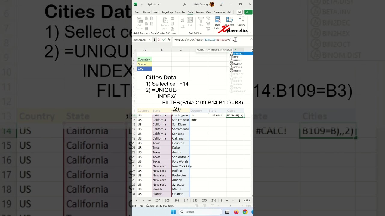
Get Unique City
1) Sellect cell F14
2) =UNIQUE(INDEX(FILTER(B14:C109,B14:B109=B3),,2))

The formula is the same as before except that we are using State in cell B3 as a condition and we are using data range from G2 to H97.

Let's breakdown the formula.
=UNIQUE(INDEX(FILTER(A14:B109,A14:A109=B2),,2))

FILTER(A14:B109, A14:A109=B2): The FILTER function is used to filter data in a range based on a specified condition. In this case, it filters the range A14:B109 based on the condition that the corresponding cells in column D (A14:A109) are equal to the value in cell B2.

INDEX(..., , 2): The INDEX function returns a value or array of values from a specified range. In this case, we are using the FILTER result as the first argument. The ", , 2" means we want to retrieve the values from the second column of the filtered range, which is column E (the first column is column D).

UNIQUE(...): The UNIQUE function is used to get unique values from a range or array. It takes the result from the INDEX function (which already contains the values from column E that meet the condition in column D) and returns only the unique values from that range.

In summary, the entire formula finds all the unique values in column E (in the range A14:B109) where the corresponding cells in column D (in the range A14:A109) are equal to the value in cell B2.

#tip #excel #microsoft #shorts #short #shortvideo #shortsvideo #howto #how #google

[bali]

Only seen a handful of your shorts, but they've each one been gems. Highly practical use cases that show a simple way to achieve advanced results. Might be worth having a related video explain the formula and functions of each short in detail, so as to advance the viewer's own understanding. Otherwise, Thank you. And I hope you keep up the good work.

[JsJs]

Nice one! Thanks for this rapid lesson!

[aniruddhapatil]

Can these dropdowns be made using only the first 3 columns?

I don't want to show the unique lists again shown in the last 3 columns.

[ArturoRuiz-]

Can you share the link to that video to make thus in rows?

[ananddwivedi]

Nice, but how can I continue this in rows so that I can use it in table forms. Is it possible??

What you shown will work awesomely for 1 row.

[NimishP]

Not sure why don’t we resort to relational database, where this can be handled very easily.