filmov
tv
How to user the Financial Functions PMT, IPMT, PPMT
Показать описание
In the current worksheet we see all the information about a personal loan.
Mr. Han has taken a loan of 120.000 dollars with an annual interest of 5.3%. The installments of this loan are to be paid at the beginning of each month for a period of 11 years.
All the other data on this sheet originate from this information. We can calculate the installment amount and we can produce a list of all our payments. We can even derive the amount of each installment that pays the interest of our loan and the amount that pays the actual principal, for each month.
The three EXCEL functions we have used here are the PMT, the IPMT and the PPMT.
These functions can be used for both loans and investments. For this reason, there is a cash flow convention.
Outgoing payments (the payments Mr. Han has to make) are represented by negative numbers and incoming payments (the payments the bank has to make) are represented by positive numbers.
Let’s go to the next sheet.
We can see again the details of a loan to Mr. Han. This time he has 2 options.
The differences between the first and the second option are that the payments are due at the end of the month instead of the beginning and he has to be able to repay an extra 3000 dollars at the end of the last month.
Why does it matter if the payment is due at the beginning or the end of a month?
At the beginning of the month the lender is getting the money earlier, thus monthly payments are less than the end-of-month case.
More so because $3,000 of the loan is not being paid with monthly payments, it makes sense that the monthly payments are less.
So let’s calculate our installment amount.
We select cell b9 and type the equals sign and the function PMT. The first argument is the rate which we can derive from cell b3. In cell b3 we have the annual interest but the installments are once per month since there are 12 installments in one year. So the rate we should type in the function is b3 divided by b6 to have the monthly interest rate. Next we have to type the total count of payments we have to make. The duration of the loan is 11 years and the installments per year are 12 so the payments are b5 multiplied by b6. Next is the present value, which means the amount of the loan in cell b2. After that is the future value which is the extra amount paid at the last month, so it is cell b7 and finally we type 1 which means that the payments are due at the beginning of the month. We press enter and we have the monthly installment of the loan for option 1.
We do exactly the same for option 2. We type “equals PMT, the rate, number of periods, the present value”. In the future value we use cell c7 which is the 3000 dollars Mr. Han will give to the bank at the last month, and finally we type 0 since the payments will be due to the end of the month.
Take note that the amount we calculated is a negative number since Mr. Han will have to pay this money to the bank.
Let us go to the next sheet. At the leftmost table we see Mr. Han’s loan information, and on the rightmost a list of all his due payments. We can see the payment number, the date it is due and the installment amount. We will now complete the rest of the table.
The next column should show the amount of the installment used for paying the interest and the last one the one used to pay the principal.
IPMT stands for Interest Payment, and PPMT for principal payment. They take the exact same arguments as the PMT function.
So in cell G2 we type equals IPMT followed by the proper arguments as before. Rate, number of periods, present value, future value, and type.
The same in cell h2 for PPMT. We type equals PPMT followed by the rate, number of periods, present value, future value, and type.
We select the two cells and autofill the entire table.
Now column G shows us the amount paid for interest and column H the amount paid for Principal.
Mr. Han has taken a loan of 120.000 dollars with an annual interest of 5.3%. The installments of this loan are to be paid at the beginning of each month for a period of 11 years.
All the other data on this sheet originate from this information. We can calculate the installment amount and we can produce a list of all our payments. We can even derive the amount of each installment that pays the interest of our loan and the amount that pays the actual principal, for each month.
The three EXCEL functions we have used here are the PMT, the IPMT and the PPMT.
These functions can be used for both loans and investments. For this reason, there is a cash flow convention.
Outgoing payments (the payments Mr. Han has to make) are represented by negative numbers and incoming payments (the payments the bank has to make) are represented by positive numbers.
Let’s go to the next sheet.
We can see again the details of a loan to Mr. Han. This time he has 2 options.
The differences between the first and the second option are that the payments are due at the end of the month instead of the beginning and he has to be able to repay an extra 3000 dollars at the end of the last month.
Why does it matter if the payment is due at the beginning or the end of a month?
At the beginning of the month the lender is getting the money earlier, thus monthly payments are less than the end-of-month case.
More so because $3,000 of the loan is not being paid with monthly payments, it makes sense that the monthly payments are less.
So let’s calculate our installment amount.
We select cell b9 and type the equals sign and the function PMT. The first argument is the rate which we can derive from cell b3. In cell b3 we have the annual interest but the installments are once per month since there are 12 installments in one year. So the rate we should type in the function is b3 divided by b6 to have the monthly interest rate. Next we have to type the total count of payments we have to make. The duration of the loan is 11 years and the installments per year are 12 so the payments are b5 multiplied by b6. Next is the present value, which means the amount of the loan in cell b2. After that is the future value which is the extra amount paid at the last month, so it is cell b7 and finally we type 1 which means that the payments are due at the beginning of the month. We press enter and we have the monthly installment of the loan for option 1.
We do exactly the same for option 2. We type “equals PMT, the rate, number of periods, the present value”. In the future value we use cell c7 which is the 3000 dollars Mr. Han will give to the bank at the last month, and finally we type 0 since the payments will be due to the end of the month.
Take note that the amount we calculated is a negative number since Mr. Han will have to pay this money to the bank.
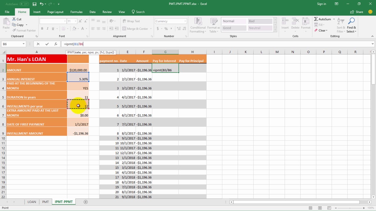
Let us go to the next sheet. At the leftmost table we see Mr. Han’s loan information, and on the rightmost a list of all his due payments. We can see the payment number, the date it is due and the installment amount. We will now complete the rest of the table.
The next column should show the amount of the installment used for paying the interest and the last one the one used to pay the principal.
IPMT stands for Interest Payment, and PPMT for principal payment. They take the exact same arguments as the PMT function.
So in cell G2 we type equals IPMT followed by the proper arguments as before. Rate, number of periods, present value, future value, and type.
The same in cell h2 for PPMT. We type equals PPMT followed by the rate, number of periods, present value, future value, and type.
We select the two cells and autofill the entire table.
Now column G shows us the amount paid for interest and column H the amount paid for Principal.
 0:06:23
 0:02:27
 0:01:50
 0:04:04
 0:00:50
 0:04:15
 0:03:03
 0:00:38
 0:00:33
 0:03:37
 0:03:20
 0:10:41
 0:05:48
 0:06:44
 0:11:32
 0:11:51
 0:14:03
 0:00:22
 0:05:45
 0:04:57
 0:01:42
 0:02:38
 0:02:50
 0:10:01