filmov
tv
Freeze Multiple Rows and or Columns in Excel and Google Sheets | Freeze Panes and View Option

Показать описание
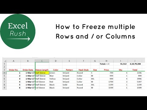
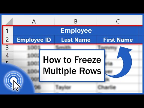
You can freeze multiple rows and/or columns in Microsoft Excel and Google Sheets to keep them visible as you scroll through your data. This is known as "freezing panes" and can be done as follows:
For Microsoft Excel:
Select the row or column below or to the right of where you want to freeze the panes.
Go to "View" in the top menu and select "Freeze Panes."
Choose one of the following options:
"Freeze Panes" to freeze the rows above and the columns to the left of the selected cell.
"Freeze Top Row" to freeze the top row.
"Freeze First Column" to freeze the first column.
For Google Sheets:
Select the row or column below or to the right of where you want to freeze the panes.
Go to "View" in the top menu and select "Freeze."
Choose one of the following options:
"Freeze 1 Row" to freeze the first row.
"Freeze 1 Column" to freeze the first column.
"Freeze 2 Rows" to freeze the first two rows.
"Freeze 2 Columns" to freeze the first two columns.
Note: In Google Sheets, you can only freeze up to the first 10 rows or columns.
To turn off freeze panes in both Microsoft Excel and Google Sheets, go to "View" in the top menu and select "Freeze." Then choose "No rows" or "No columns."
=====================================================
freeze panes and view option
how to freeze panes in excel
freeze rows and columns in excel
freezing multiple rows and or columns in excel
how to freeze rows and columns in excel
freeze panes in excel column and row
how to freeze row in excel
freeze multiple rows and or columns in excel and google sheets
freeze rows in google sheets
freeze rows and columns in excel
freezing multiple rows and or columns in excel
how to freeze rows and columns in excel
how to freeze multiple rows and or columns in excel
how to freeze multiple rows and columns in google sheets
how to freeze rows and columns in google sheets
how to freeze panes in excel
hasan academy
=====================================================
COMMUNICATE WITH HASAN ACADEMY
Facebook page
Комментарии
 0:02:01
 0:00:34
 0:02:45
 0:03:35
 0:01:00
 0:00:51
 0:02:16
 0:00:18
 0:00:16
 0:03:46
 0:01:21
 0:00:53
 0:02:06
 0:01:06
 0:01:15
 0:03:44
 0:03:49
 0:02:33
 0:02:02
 0:02:31
 0:01:26
 0:04:06
 0:00:15
 0:01:38